HuggingArch: Automating Model Architecture Analysis

I spent the better part of a year's worth of spare time on this project. If you find it interesting or useful, please give it a star and come be a developer. I haven't quite figured out a sensible way to co-build a vibe-coded project yet, and that's something I'd love to talk through with anyone who has ideas.

TL; DR

HuggingArch has an agent automatically write an open-source model up as a structural description (a DSL spec), then runs LLM deployment analysis on that spec automatically.

• Website: huggingarch.com
• Code: GitHub

It's probably the first framework that does deployment "cost accounting" automatically. You can think of it as a peculiar compiler: the HuggingFace config is the input, the spec is the IR, graph compilation handles shape propagation, parallel sharding and operator fusion, and sympy plays the runtime. The difference is that it doesn't compute real tensors; it computes FLOPs, memory traffic and memory footprint. All you provide is a HuggingFace model ID, and the agent generates a description of the model's structure. Everything after that, shape propagation and graph rewrites, is deterministic, and one click gives you the model's theoretical performance across parallel configurations and GPU types. That makes comparing different model architectures very lightweight.

1. Intro

HuggingArch is a project that tries to use a harness approach to automate cost accounting for LLM inference, for any model that's open-sourced on HuggingFace. The motivation is pretty straightforward. There are more and more models, and as practitioners we constantly need to analyze and compare their strengths and weaknesses. That's a critical issue for model labs, MaaS providers and chip vendors alike. Cost accounting is laborious, and the bar isn't exactly low. Over the past year, model labs went all-in on hybrid architectures and model structure got far more diverse, which actually makes the math harder: Is DSA or KDA cheaper at long context? How much do CSA and HCA save compared to DSA? Is DeepSeek really supposed to be this cheap? How much more will K3, as a 3T-class model, cost? Just thinking about these questions feels like weeks of work. To keep our own working memory from OOM-ing, it's 2026, and we really have to get an agent to do the math for us.

Right now the project covers computation-graph visualization of model architectures and theoretical cost accounting for LLM inference, and the backend also directly supports benchmarking operator performance across frameworks (extremely simple to use), so you can quickly get real performance numbers for a specific deployment. In fact, HuggingArch can also turn each model's modules into pluggable units. A Model Arch Designer can then freely change hyperparameters, arrange different module units into a new model, and quickly work out what that model costs on different GPU types and deployment setups. That's the most interesting part of standardizing models into a composable DSL.

Since this is purely a side project, it took the better part of a year to go from the first idea, through all the refactors, to finally feeling it was actually usable enough to put out there. I kept patching it together in scraps of time after work and on weekends. Meanwhile, model architectures got more and more complex over those months, and the syntax needed to express them kept growing. Today, using a frontier model to quickly analyze a model's KV cache and theoretical FLOPs is no longer hard. So what's the point of this project? In short, I think it's a trustworthy, self-correcting, reusable, lightweight piece of infrastructure.

• Trustworthy: analyzing a model purely by vibe is ad hoc. You have to carefully trace back through the agent's computation before you dare believe the result. And agents, by habit, are better at telling you the answer than showing you the intermediate steps. Without feedback, expecting an agent to go all-in on one turn and produce the right answer is unrealistic, and the more complex the model, the lower the odds of getting it right. Human feedback is a very inefficient process. Is there a mistake? If so, where? On one hand, the analyst has to already be familiar with the architecture to correct the model; on the other, repeatedly grilling the agent just makes the session longer and longer, and the shifting answers feel less and less trustworthy.

• Self-correcting: HuggingArch has a validation system built on ground-truth information such as the model's original forward code, its config and its weights, which lets the model correct itself, so nearly all the low-level mistakes get eliminated. On top of that, every computation in the system is built on sympy's symbolic system, so every value comes from a specific formula, and those formulas pass straight through from the backend engine to the frontend, which means any error in any formula can be spotted by a human.

• Reusable: every model goes into the repository as a spec. Specs are abstracted into three levels: primitive, component and model. So components shared across models, like Attention and MoE, can be reused across models. This lowers the difficulty of generating a spec for a model, reduces ambiguity in the computation, and keeps the repository's entropy growth within a fairly controllable range. Once models are assembled in the repository out of modules, in principle I can give them almost the full capabilities of a Graph Compiler: shape propagation over the computation graph, quant, activation liveness analysis, device mapping. The only difference is that underneath, it doesn't do actual tensor computation; it computes FLOPs and memory traffic. And so a simple, agent-driven spec grows into a complex model analysis system.

• Lightweight: none of the analysis needs the model to run. So no operator implementations, no framework runtime, no GPU. That means models of any size can be analyzed quickly, and every result stays traceable over the long term.

An LLM inference cost-accounting system needs two essential ingredients:

1. A representation of the model architecture

You could build it by hand, but rebuilding a model manually is still a hassle, and an agent can do the writing just fine. The most direct information the agent needs to build this is: the shapes of the model weights, the structure of the computation graph, and the model's parameters. HuggingFace happens to have all of it: the model weights, the transformers library and the inference source code. So our web system is built on HuggingFace, but there's also a backend CLI tool you can DIY with (vLLM/SGLang source code and model weights work too).

Why an agentic approach to generating models?

The goal was clear from day one: build a lightweight analyzer that works across models. Downloading weights is out, since they easily run to several TB and there's no way to do that concurrently. Actually running the model is out too: GPUs are too expensive, and the various CUDA and inference-engine versions are too heavy. The most obvious idea was to use transformers' meta device to "dry-run" the model: hook in before each layer runs to compute FLOPs, and get the structure from graph analysis. As it turned out, not a single runtime-dependent route worked:

1. The meta device can build a model but can't run forward. init_empty_weights() plus from_config gets you a structurally complete nn.Module with no weights, but the moment it actually computes anything it errors out. For example, some models call .cpu() inside forward.
2. Extracting the computation graph from PyTorch means retracing PyTorch's whole compilation path. torch.export can't handle data-dependent control flow, and the exported ops are too fragmented to read. Trace / dynamo need constructed inputs, but every model's forward signature is different (KV cache, position encodings, top-k indices… each passes its own), so it's hard to fabricate valid data. Analyzing the AST directly drags you into a mass of Python language-level details.
3. transformers' backward compatibility is poor, and model code itself often won't run. For example, transformers 5.x changed the RoPE config from a flat rope_scaling to a nested rope_parameters, and MiMo-V2-Flash, written against 4.x, just errors out. Even if you dynamically switch transformers to the version written in each model's config.json, you run into other dependencies. Kimi's modeling code, for instance, imports flash_attention directly and won't start in a CPU environment.

Since the runtime route was a dead end, we arrived at the current approach: don't run any existing runtime, just have an agent write the spec.

2. A methodology for inference cost accounting

Speed-of-Light estimation is the computational foundation of this project. LLM inference consists of two phases, prefill and decoding. Each phase's compute pattern is determined by the operators that dominate its forward time. The former is generally compute-bound, because GEMM and Attention operator shapes have good roofline AI (arithmetic intensity), so GPU TFLOPS bounds the lower limit of its execution time. In the latter, GEMM and Attention operators are generally memory-bound, so memory bandwidth bounds the lower limit of its execution time. A good reference for the definition of this metric is SOL-ExecBench: Speed-of-Light Benchmarking for Real-World GPU Kernels Against Hardware Limits.

$$T_{\mathrm{SOL}}=max(\frac{\text{Total FLOPs}}{\text{Compute Throughput}},\frac{\text{Total Fused Bytes}}{\text{Memory Bandwidth}})$$

From each operator's $T_{sol}$, we can propagate bottom-up through the computation graph to derive the SOL time of the prefill/decode phases, and from that get a cost estimate for inference.

1.1 Core architecture

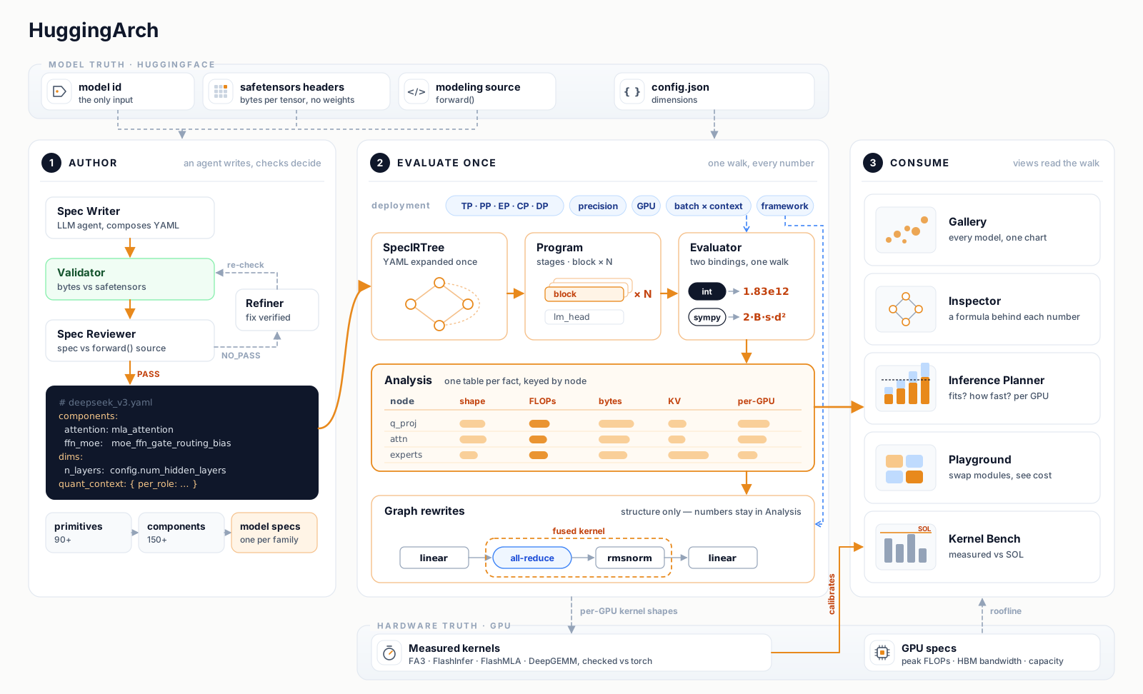
The top and bottom layers are external facts; the three steps in the middle are the system itself:

• Model truth: the config, safetensors headers and modeling source code on HuggingFace are the system's only input.
• ① Author: the agent writes the spec, then deterministic checks gate it. Only when the bytes match the checkpoint and the semantics match the source code does it go into the repository.
• ② Evaluate once: the spec is evaluated exactly once, producing shapes, FLOPs, memory and per-GPU sharding. Communication and fusion only rewrite the graph; they don't recompute.
• ③ Consume: every page reads the results of this one evaluation, so the same number is the same wherever you look at it.
• Hardware truth: kernels are measured at real per-GPU shapes and used to calibrate the estimates.

The details of each part are covered in Chapter 2 (spec) and Chapter 3 (inference cost accounting).

---

2. Building the model spec

The core of HuggingArch's architecture is a bottom-up DAG DSL, plus the SpecTree IR built on top of that DAG. Claude Code writes the DAG; the SpecTree IR is built-in framework code. That way the agent always exercises its ability to turn unstructured data into structured data inside a set of constraints. It's worth stressing again: the computation graph is the core abstraction of today's deep learning frameworks, and the transformer is just one particular structure built on that abstraction. A well-built computation graph can, in theory, represent any model structure, however complex. Hang the Sympy symbolic math system on this IR and you can express structural relationships, shapes, and arithmetic all at once. Once you have that description of the computation graph, higher-level, task-specific computations on top of it (say, deriving inference KV cache capacity, or deriving parallelism) are just application layers on the spec system.

2.1 The core: the spec system

HuggingArch builds the model structure by reading the inference source code in transformers or in the model's official repo. Reading code is an open-ended problem, so we need a well-defined DSL that tells the agent (e.g. Claude Code) how to write it and what the result should look like.

1) Three levels of op: Primitive / Component / Model

• Primitive ops are the lowest-level operators (linear, rmsnorm, rope, attention_score, ...), built into the framework. Each primitive op carries three things: a parameter-count formula, a FLOPs formula, and a shape rule. The formulas are sympy expressions directly; for example, the matmul in linear is 2·B·s·in·out.
• A Component is a DAG made of primitive ops or other components, written in YAML. Most of the diversity in model structure lands at this level: GQA, MLA, SwiGLU, MoE, and DeepSeek-V4's CSA are all components. Reviewed components go into library/ for every model to reuse; new ones the agent writes start in drafts/, visible only to the spec that declares them, and are merged into the library after they pass review.
• A Model fills components into block templates, then says which template each layer uses. A hybrid model is just one where different layers use different templates.

Take DeepSeek-V3's MLA as an example. One structure is assembled from three declarations (all excerpts):

# components/library/mla_attention.yaml — component: a DAG
role: attention                          # can fill the attention slot of a block template
cache:                                   # what's kept across steps during decode
  family: MLA
  entries:
    - { node: kv_a_layernorm, kind: latent }     # the compressed KV latent
    - { node: k_pe_rope,      kind: rope_key }   # the rope key shared by all heads
decode_variant: mla_attention_absorbed   # at decode, swap in a subgraph that computes in latent space
graph:
  kv_a_proj_with_mqa: { op: linear, in: x, dims: { in: d_model, out: "d_kv_lora + d_qk_rope" },
                        weight_axes: [{ replicated: true }, { replicated: true }] }
  kv_latent_slice:    { op: slice, in: kv_a_proj_with_mqa, dims: { in: "d_kv_lora + d_qk_rope", out: d_kv_lora } }
  kv_a_layernorm:     { op: rmsnorm, in: kv_latent_slice, dim: d_kv_lora }
  kv_b_proj:          { op: linear, in: kv_a_layernorm, dims: { in: d_kv_lora, out: "n_heads * (d_qk_nope + d_v_head)" },
                        weight_axes: [{ world: attention, parts: n_heads, fit: replica_cells }, { replicated: true }] }
  # … Q compression and decompression, head split, rope, attention_score, softmax, attention_apply, head merge
  o_proj:             { op: linear, in: o_merge_heads, dims: { in: "n_heads * d_v_head", out: d_model },
                        weight_axes: [{ replicated: true }, { world: attention, parts: n_heads, fit: replica_cells }] }
outputs: [o_proj]

# models/deepseek_v3.yaml — model spec: fill components into slots, take dims from config
components:
  attention: mla_attention
  ffn_moe:   moe_ffn_gate_routing_bias
  block:     pre_norm
dims:
  n_heads:   config.num_attention_heads
  d_kv_lora: config.kv_lora_rank
  d_qk_rope: config.qk_rope_head_dim

# arch/dims.yaml — global dimension table: each dim is classified once, including which parallelism can shard it
n_heads:   { kind: head_count, shardable_by: [attention] }
d_kv_lora: { kind: whole }                # the latent isn't split by head, so it can't be sharded

This maps to four things:

• The role decides where it can plug in. role: attention says it can fill the attention slot of a block template, and the model spec's components: fills in the blanks by slot name. Switching to a different attention means switching the component; the block template stays put. Roles are all registered in roles.yaml, and any name not registered there is rejected at load time.
• The cache declares what's left behind during decode. MLA doesn't store per-head K/V; it stores only the compressed latent and one rope key shared by all heads. The KV cache formula is computed directly from the shapes of those two nodes: d_kv_lora + d_qk_rope elements per layer per token. decode_variant says the decode phase swaps in the "absorbed" version of the subgraph, which computes attention directly in latent space.
• Dims are symbols, and in: is a real edge. A component only writes expressions like "n_heads * (d_qk_nope + d_v_head)"; the concrete values are bound from config by the model spec. DeepSeek-V3, Kimi-K2, and LongCat-Flash use the same component, just with different dims. The engine propagates shapes along in:, and FLOPs and bytes are all computed from the propagated shapes.
• Sharding is declared in two places, and communication isn't written at all. Which parallelism can shard each activation axis is written once, in the global dimension table (head count belongs to attention TP; the latent dim can't be sharded). Weight placement is written per axis on the node with weight_axes: kv_b_proj's output axis is sharded by head, o_proj's input axis is sharded by head, and the compression projection kv_a_proj is fully replicated because the latent isn't split by head; fit says how to split when the head count doesn't divide evenly by the GPU count. Collectives don't need to be declared: the activation layout propagates along in:, and wherever the layouts on either side don't line up, the engine automatically inserts communication such as all-reduce.

Encapsulation can't be finer-grained than the source. An agent will happily inline a standalone function from the source (DeepSeek-V4's hc_pre, for example) into a pile of atomic ops: the structure is right, but the semantics are lost, and the resulting graph is unreadable. So we require the spec's encapsulation granularity to be ≥ that of the source's forward(). It can be more abstract than the source (folding an implementation reused in several places into one component), but never more fragmented.

For the full syntax and design trade-offs, see docs/design.md.

2) A symbol system across all three levels

I want HuggingArch to give you not just numbers but explainable formulas. A black-box planner hides its assumptions in code details, and LLM infra techniques keep changing. I don't demand that the cost accounting system can model everything, but I do need to know what assumptions it made, so I can judge how far to trust its numbers. That's why hovering over any value in the frontend shows the symbolic expression behind it.

The way to do this is to have all three levels share one dimension environment: primitive op formulas take their symbols from it (d_model, n_heads, batch B, this step's sequence length, ...), nested components pass the binding down layer by layer, and the whole graph ends up as one sympy expression tree.

Dual-track evaluation is the biggest payoff of this design. In the same walk, bind numbers and you get a number; bind symbols and you get a formula (2·B·s·d_model²). There's only one engine; "number or formula" is a property of the binding, not a code branch, so the formula and the number can't disagree.

Heterogeneous layers aren't flattened. A hybrid model's totals are kept as sums, e.g. n_dense·MLA + (n_layers − n_dense)·MHA, and KV cache, weights, and memory traffic are each summed separately.

But the symbol system only answers "how is this number computed"; it doesn't prove "is the graph itself right". That falls to the checkpoint anchor below (which must pass before publishing) and the forward / shape checks (best-effort diagnostics). The two are guarantees of different strength.

2.2 Handling complex hyper-connections: the stream mechanism

A classic Transformer has exactly one inter-layer connection: the residual. Layer l's output is layer l+1's input, so the spec just writes repeat: n_layers and the engine unrolls by layer count. Models in the last couple of years are no longer content with that single line, and more and more values "hop" between layers:

• DeepSeek-V4's Hyper-Connections: the residual goes from one copy to n_hidden_copies parallel copies, and each layer does a learnable n→1→n mix before and after attention / FFN;
• Qwen3-VL's DeepStack: the intermediate hidden states from layers 8/16/24 of the vision encoder each pass through a merger, then are added onto the visual-token positions of the outputs of layers 0/1/2 of the language model, respectively;
• Kimi-K3's AttnRes: every Kar layers, the hidden at the layer entry is saved into a history, and every later layer does an attention-style weighted merge over the whole history, instead of just adding the previous layer's residual;
• GLM-5's DSA index sharing: the top-k selection computed by a full layer is passed via prev_topk_indices all the way to the later shared layers for reuse;
• YOCO (You Only Cache Once) / CLA (Cross-Layer Attention): later layers read some earlier layer's KV cache directly instead of computing their own;
• Llava / EAGLE-3: take the hidden states from several layers, concatenate them, and hand them to a projection layer or a speculative decoding head.

If we added a dedicated spec field every time we hit one of these, the DSL would grow longer and messier, and the agent wouldn't remember which field to use for which case. Looking back at these structures, they're really all the same thing: a value is produced in some layer iterations and consumed in others. So HuggingArch keeps just one concept to describe all cross-layer dataflow: the stream.

1) Every cross-layer value is a stream, declared on the layer stack

The most common one, the residual itself, is also a stream; there's no implicit default channel. A repeated layer stack explicitly declares the trunk it passes from layer to layer:

- name: layers
  repeat: n_layers
  inputs: [embed_tokens]
  streams:
    hidden: { carries: true }   # the trunk passed layer to layer; TP sharding is gathered at each layer exit automatically, no extra declaration needed

DeepSeek-V4's Hyper-Connections don't need a new mechanism: the shape of hidden is simply [B, s_ctx, n_hidden_copies, d_model]. At the entry, hc_expand copies the embedding n times; inside each block, two components, hc_pre / hc_post, do the n→1→n mixing; at the exit, hc_head folds it back to one copy. A "multi-copy residual" is just the trunk stream with a different shape, not a new kind of connection.

The remaining cross-layer values fall into two kinds, by "who produces it and who reads it".

Internal streams: produced by some node inside a layer, read by some node inside a later layer. GLM-5's DSA index sharing works like this: the stack declares the stream name, the full layer's attention component publishes the top-k selection with stream_out, and the shared layer's attention component reads it with reads:

# models/glm_moe_dsa.yaml — declare the stream on the layer stack
streams:
  hidden: { carries: true }
  dsa_topk:
    shape: [B, s_query, n_topk_keys]
    src: "GlmMoeDsaAttention.forward threads `prev_topk_indices` across layers"

# components/library/mla_dsa_attention.yaml — full layer: publish the computed top-k to the stream
stream_out: { dsa_topk: dsa_topk_mask }

# components/library/mla_dsa_attention_shared.yaml — shared layer: read the stream instead of computing it
reads: [dsa_topk]

The src on a stream is where this cross-layer channel comes from in the source: a one-line description plus a real code snippet in backticks (here, prev_topk_indices). Validation looks it up in this model's forward() source; if it isn't found, that's an error and the spec can't be published. Every cross-layer channel a spec claims must be backed by something in the source.

YOCO / CLA are written the same way: the writer stream_outs the KV node it caches, and the reader reads it. The engine follows the stream to its single producer; the reader's memory traffic is counted into kv_reads according to the cache's own growth rule and dtype, and the cache is stored only once.

Append streams: "save" a value on selected iterations and accumulate a sequence for someone else to read. The declaration says where to take it from (from) and on which iterations (after takes it at the layer exit, before at the layer entry); the reader then decides how to read it:

Read mode	Meaning	Example
read: each	The j-th reader reads the j-th element	Qwen3-VL DeepStack
read: all	Each layer reads the full history accumulated before it	Kimi-K3 AttnRes
read: concat	Concatenate along some axis and read as one tensor	Llava multi-layer features, EAGLE-3 auxiliary hidden

Qwen3-VL's DeepStack uses append streams twice in a row: the vision stack saves hidden after layers 8/16/24, and the merger stack reads them in one by one; the merger outputs are then accumulated into deepstack_feat, which the first three layers of the language model read one by one:

- name: visual.blocks
  repeat: n_vis_layers
  streams:
    hidden: { carries: true }
    deepstack: { from: hidden, after: config.vision_config.deepstack_visual_indexes, index: block,
                 src: "if layer_num in self.deepstack_visual_indexes:" }
- name: visual.deepstack_merger_list
  repeat: n_deepstack                    # must equal the number of elements in deepstack
  inputs: [deepstack]                    # iteration j binds element j
  streams:
    deepstack_feat: { from: out, after: every, index: block,
                      src: "deepstack_feature_lists.append(deepstack_feature)" }
- name: language_model.layers
  repeat: n_layers
  streams:
    hidden: { carries: true }
    deepstack_feat: { read: each }       # the injection nodes of the first n_deepstack layers read them one by one

Kimi-K3's AttnRes is before + read: all:

streams:
  hidden: { carries: true }
  block_residual:
    from: hidden
    before: { every: Kar }               # entries of layers 0, Kar, 2·Kar …
    read: all                            # each layer reads the full history accumulated before it
    src: "block_residual = torch.cat("

read: all means different layers see histories of different lengths (layer l sees ⌈l/Kar⌉ entries), so their shapes and FLOPs differ too. The engine splits that one declaration into groups by "visible history length" and evaluates each group separately; for display, it merges them back into a single card by declaration and shows the "history length → layer index" distribution. The computation is exact, and the page still shows 3 or 4 kinds of layer rather than a thousand-plus rows.

2) Why it's designed this way

• One concept covers every case. None of the six structures above needs a dedicated field. When a new model shows up with yet another cross-layer connection, odds are it's just a new combination of "where from, on which iterations, how it's read".
• One place to declare. Streams are declared only on the layer stack; when a node inside a component needs to read or write one, the component binds it with reads / stream_out. To see a model's cross-layer structure, you only need to read its model: section.
• Every stream carries a source anchor. src: cites the line in the forward source that produces or consumes the value, and validate checks it like any other source anchor, so a spec can't conjure a dataflow that doesn't exist in the source.
• Constraints belong to the schema. A mis-written stream errors out right at load or validate time, with the correct form in the error message, and goes back to the generating agent as a fixable error. For example, trying to use slice to "take layer i's output" from a layer stack actually only reads the last layer; that form is rejected, with a hint to use an append stream with after: [i] instead. The generation prompt contains only a positive "forward pattern → stream pattern" lookup table, no list of don'ts.

2.3 Sources of truth: where the ground truth comes from

To make spec generation both accurate and cheap, HuggingArch pulls information from several sources of truth for an HF model, without downloading any weights at all:

• config.json: via _fetch_config() in backend/analyzer.py, which tries, in order, the local custom-model cache, the built-in snapshots (backend/arch/snapshots/), and an online download from the HF Hub. This is the scalar source for model sizes (d_model / n_layers / n_heads / d_ffn / n_vocab, etc.).
• Printed model skeleton: _fetch_model_str() uses init_empty_weights() to build an empty model on the meta device, then print(model) to get the module hierarchy tree. This step doesn't download weights or run forward; it's only there to get the nested nn.Module name structure and shape annotations. The result is cached in ~/.cache/huggingarch/model_info/.
• forward source: backend/hf/forward_source.py tries, in order, the snapshot, the custom model, inspect.getsource() on the local transformers, the model-info cache, and the source files in the HF repo, and hands whatever implementation it gets to the spec generation agent; it's also used by the best-effort AST structural diagnostics.
• safetensors index: backend/hf/metadata.py (a fairly large module) uses just 2–3 HTTP range requests to fetch model.safetensors.index.json and the metadata block of each shard, getting each tensor's name, shape, dtype, and storage bytes without downloading a single weight byte. This is the ground truth for the parameter-count + bytes check.

For private repos that aren't in mainline transformers and are only provided via trust_remote_code in the model card (typically Kimi, MiMo, GLM-MoE, etc.), HuggingArch pulls modeling_*.py and configuration_*.py from the model repo on the HF Hub and feeds the forward source to the agent. When it hits a native dependency like flash_attn, it doesn't actually import it; it just reads it as text. That sidesteps the "can't run it at runtime" problem.

These inputs go down two paths of different strength: the forward source and model skeleton help generation and produce non-gating structural diagnostics, while the safetensors metadata feeds the total-bytes and tensor-coverage gate.

2.4 Shape inference: geometric consistency inside the spec

When an agent writes a spec, the easiest mistake to make isn't a wrong parameter count; that kind of error is easily caught by the tensor comparison described later. The easiest mistake is a geometric error: forgetting to broadcast MLA's k_pe to all heads before concatenating, doing a view_split on a flat dim that isn't actually n_heads·d_head, Q and K head_dims not lining up... These errors can perfectly well cancel out in the parameter count (one linear counts a few extra parameters, another counts a few too few, and the bytes diff is still 0), but the forward dataflow is wrong. The spec appears to pass validation, yet the inference analyzer gives an absurd KV cache, the wrong attention type, and shape badges that don't line up with each other.

The fundamental difficulty: HuggingArch doesn't run the model, so how do you verify the forward topology is right?

The first version took a detour: it tried to have each component declare a shape: for every node, with the engine only checking consistency. But that path basically pushes the burden onto the spec author. For a V4-Pro block with 60 nodes, the author has to work out every node's shape and write it into the yaml, which is more error-prone than just writing the forward.

The path we ended up on makes shape inference a first-class mechanism:

1. in: isn't a comment; it's a real dataflow edge. Following each node's in:, the engine looks up the upstream output in Analysis.shapes by UID and hands it to the current op's DimMap.
2. Every primitive op declares a shape_kind. Built-in ops currently use 9 kinds (preserve / broadcast / axis_replace / axis_select / axis_concat / contract / permute / source / explicit), which the engine compiles into a DimMap for shape inference. YAML custom_ops can declare the first 7; source / explicit, which need a DimMap, must be registered as built-in ops.
3. Unified across scales: between nodes inside a component, across nested component calls, and across model layers (each layer's shape_out becomes the input for the next layer's inputs[0]), all three scales share the same dataflow propagation. A V4-style [B, s_ctx, n_hidden_copies, d_model] hyper-connection input flows through the whole graph, so the engine sees the real tensor shape and nothing downstream has to guess backwards.

Only after shape was lifted to first-class did we get the key capability: the validate stage can check geometric consistency without running any numbers. Supported rules such as axis_concat, attention_score, contract, and some multi-input add / mul check rank, non-axis dims, and relationships like the Q/K head_dim. The results go into shape_mismatches and into errors: a graph whose tensors can't be put together can't be published just because the checkpoint's total byte count happens to match.

The real value of this path is that the dataflow the spec declares for itself can be propagated and checked consistently. It catches internal geometric contradictions, but a self-consistent wrong graph can still pass, so it can't be called a local reproduction of the forward source.

2.5 Tensor weights: ground truth for parameter counts and quantization

LLMs writing specs that "look perfectly reasonable but are wrong somewhere" is an everyday thing. But as long as the weights are in the ckpt, the truth is right there: safetensors doesn't lie. Its tensor names and byte counts are facts the upstream model team put there with their own hands. The question is how to use those facts as a check.

One source of truth, two layers of information

HuggingFace tensor names follow a fairly stable convention:

model.layers.X.self_attn.q_proj.weight                         ← standard LLM
model.layers.X.mlp.experts.X.gate_proj.weight                  ← MoE
model.vision_tower.encoder.blocks.X.attn.q_proj.weight         ← vision tower
model.language_model.layers.X.self_attn.q_proj.weight          ← multimodal nesting

This naming encodes two kinds of information at once, and the validation mechanism handles them along two separate paths.

Topology information (which layer, which attention slot, which expert) is expressed by the hierarchy of the name prefix. The validator uses canonical_module_path() to normalize both HF tensors and spec leaves, then does an equality join on the canonical key; there's no separate HF normalizer and no longest-suffix fallback. In a heterogeneous stack, several spec leaves can map to the same canonical module path, and the matcher aggregates them before reconciling against the HF module.

Quantization packing information (is this a GPTQ qweight, MXFP4 _blocks, or FP8 .weight + scale_inv) is expressed by the name suffix together with the dtype. HuggingArch's strategy here is to write each quant scheme's on-disk representation as yaml: the main weight's packing factor / storage dtype / suffix, the suffix and cardinality formula of the metadata siblings, the rule for deciding the logical element format, and the scale granularity type.

That sounds mundane, but it's a deliberate boundary: tensor naming conventions and packing details are messy knowledge where "upstream transformers / autoawq / compressed-tensors / every training framework each does it their own way". That knowledge used to be scattered across several Python libraries, and every new scheme meant invasive logic in one more place. Once it's normalized into yaml, adding a quant scheme is a matter of declaring yaml, not changing Python. Every downstream consumer shares the same source of truth.

Decoupling quantization: architecture vs storage

Model architecture and quantization are two things that combine independently: the same DeepSeek-V3 has BF16, FP8, and INT4 checkpoints, and for the same checkpoint you can ask "what if I deploy it in FP4". So the spec writes them separately:

• Architecture is dtype-agnostic. linear only cares about parameter count and FLOPs; there's no dtype in the formula.
• Storage is declared separately. The spec carries a quant_context that declares the quantization scheme per role, with the few exceptions called out individually via override. For example, gpt-oss quantizes only the MoE and keeps everything else in BF16:

quant_context:
  per_role:
    ffn_moe: { method: mxfp4, group_size: 32 }
    default: { method: none }
  default_dtype: BF16

Weight bytes are computed in exactly one place, by combining geometry and format, and validation, capacity, KV, and the frontend badges all read that one result instead of each parsing HF's quantization_config on its own. Once quantization is computed separately in several places, mixed-precision models immediately stop adding up.

So the spec can answer two questions at once: what it actually is (reconcile quant_context against the real checkpoint), and what happens if it's deployed at a different precision (use a precision profile to rewrite the formats of weights, activations, matmuls, and caches; anything not rewritten keeps its factory precision). Changing precision is just re-evaluating with a different binding; no second set of computations is needed.

The hard criterion: bytes, tensor by tensor

The final hard criterion is bytes: the spec computes how many bytes each weight takes on disk and reconciles that against the per-tensor byte counts recorded in the safetensors header. We use bytes rather than element counts because in a mixed-precision checkpoint (FP4 experts + FP8 attention + BF16 norm), physical bytes are the only thing that doesn't need unit conversion. Any tensor not claimed by some spec node, and any tensor whose element count doesn't match, is an error outright. Matching total bytes is just the final checksum: it catches a wrong width, but it can't tell that two submodules swapped places.

2.6 Guards: when it's wrong, is there anything to catch it?

Let me start with a real case where things went wrong. After DeepSeek released V4-Pro, I had an agent write up the deployment cost accounting for V3 / V3.2 / V4-Pro on 8×B200: prefill, decode, max-batch, with context swept from 4K to 1M. It looked the part. The architectural differences were laid out in fine detail, the qualitative conclusions held up, and the whole thing was full of roofline formulas and sweep tables. Then I reconciled it against HuggingArch: qualitatively all correct, quantitatively it fell apart.

• For V3 prefill at 1M context, the doc said 73.48 µs/token. Recomputed from first principles it's about 150. A ×2 was missing. You'd never spot it looking at that one cell, but it was the baseline, so one error polluted the whole column: V4's prefill speedup over V3 was written as 4.7×, while the true value is 9.4×. The single biggest selling point of this model got undersold by half.
• Short context was sneakier. The doc assumed prefill is compute-bound, but single-request, short-context prefill is actually bound by moving weights: a huge pile of MoE expert weights has to be read from HBM. This isn't a copied-wrong number. It's a modeling assumption quietly breaking down in one regime.

What the agent wrote looked even more professional than what a human would write, but it couldn't find the hidden ×2 or the broken assumption on its own. Having an agent review it again doesn't save you either: hallucination reviewing hallucination only looks more correct the more you read it. So the starting point of HuggingArch is not to stop agents from doing the math, but to stop them doing it in an unconstrained vacuum: what the agent writes is a constrained spec, and at every step there are external facts that can catch it.

These "things that catch it" are the guards. They come in two strengths: ones that block publishing, and ones that only give feedback.

Guard	Checked against	Which errors it catches
weight	Name, shape, and bytes of every tensor in the safetensors header	A tensor not claimed by the spec; element count or bytes don't match; total bytes don't equal the file's actual bytes
packing	Quantization packing scheme	Stored element count and dtype each wrong (two errors cancel out and total bytes happen to match); a quantization override that hits no tensor
shape	The spec's own dimensions and op rules	Tensors that don't fit together
analysis	The evaluation itself	The spec can't complete one evaluation
schedule	Per-layer lists and parameter values in config.json	The per-layer schedule doesn't cover every value that appears in the list; a parameter specified in config isn't bound to its op
structural	RoPE segments and each attention's mask in config	Rotary position embedding segments or causal / bidirectional masks disagree with config; a parameter declared but never used
axiom	Per-layer invariants written by the component author (how KV grows, how big the sliding window is), cache declarations	Evaluation results disagree with the declaration; config declares a sliding window but the spec has no capped cache; a cache's read/write pattern contradicts itself
source	forward() source code	A cross-layer stream's source anchor can't be found in the source, or it has no producer / reader

Every row above blocks publishing. There's another batch of checks that only give the agent feedback and don't block publishing: comparing the call order and residual count of forward() via AST, running each module as a trial, whether the activation function matches config, whether the parameter count matches the model card, and whether drafts duplicate each other.

Whether something can be published depends on one thing only: whether the errors returned by validate() are empty. Two boundaries should be stated clearly too. First, each of these checks handles one class of error, and together they still can't prove the spec is fully equivalent to forward. Shape only says the tensors fit together; the AST comparison only compares call order and residual count. Semantic alignment relies on the review in section 2.8. Second, the schema only blocks wrong references and unregistered roles. It doesn't block new topologies: when the agent meets a structure that isn't in the library, it just inlines a new block in its own spec. The cost of a new topology should be "write a new YAML", not "change the library first".

Are guards really necessary? We ran a controlled experiment (full report at docs/guard_ablation/report.md): an agent (Claude Opus 4.8) rewrote the specs for three models from scratch in a decontaminated sandbox. The target's own components, all same-kind components in the library, and every other spec were removed, leaving only the generic building blocks plus the target's source, config, and tensor names. Then we added the guards back one tier at a time, from all off upward, with 3 seeds per tier.

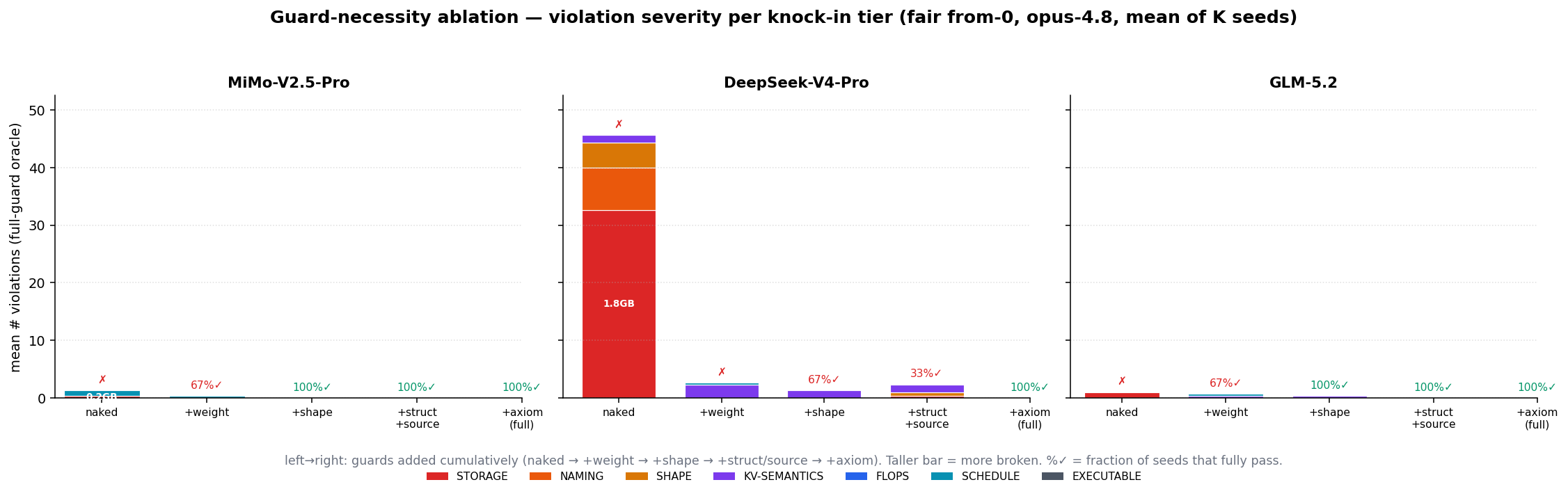
Model	All off (no guards)	All on
DeepSeek-V4-Pro (1T, Hyper-Connections)	0% pass: 32.7 storage errors on average, 1.8 GB byte gap	100% pass
GLM-5.2 (MLA + DSA + MoE)	0% pass: storage errors	100% pass
MiMo-V2.5-Pro (sliding window + fused QKV)	0% pass: storage and per-layer schedule errors	100% pass

Each guard added back eliminates its corresponding class of error. The most notable thing is what failure looks like: at the all-off and weight-only tiers, the agent reports success when it exits, and its own weakened validation is green too. It thinks it's done, yet when the fully-on validation runs, the spec is broken. In another experiment across 8 different coding agents, with all guards off, 94% of the broken specs were self-judged "passing" by the agent; with all guards back on, that dropped to 6%. The harder a model is to derive, the more it needs guards: deriving V4-Pro from scratch takes 62–87 turns, 44–63 minutes, and 14–22 dollars, 3–4× the other two models, and it also produced the most outrageous errors. (These experiments ran on an earlier version. The current implementation added an overlapping check for sliding windows, so the claim that "each guard uniquely catches one class of error" has to wait until the experiment is migrated and rerun to be confirmed.)

So what HuggingArch wants to solve was never just the manual-labor problem of "not having to hand-build every new model". It's the trust problem of "can the agent's math actually be trusted". Getting a model to generate an analysis is too easy. The hard part is getting it to generate a trustworthy one: lay out the formulas and assumptions, pin the verifiable parts to external facts, and explicitly hand the rest to diagnostics and review. Only a system like that has standing to discuss whether a sentence like "V4 is 9.4× faster than V3" can safely go out.

2.7 How a new model's spec is generated

Back to the original goal: "input an HF model ID, output a verified spec". backend/spec_worker/ orchestrates this as an agentic pipeline. The vast majority of new models are, topologically, combinations of existing components (a hybrid GQA + MLA, SwiGLU + 256-expert MoE, add a sliding window, swap the RoPE). The agent just fills role slots like attention / ffn / norm in the model spec with ready-made components; existing adapters/ shims can carry pure binding and checkpoint-naming differences. When there really is a novel topology (like DSv4's hyper-connection, CSA's sparse indexer, SSM), the agent writes a new component in components/drafts/ and lists it explicitly under drafts: in the model spec. After review passes, a maintainer can run python -m backend.arch.promote <name> to git mv it into the library; an unreviewed draft is only visible to the spec that declares it and doesn't pollute the global manifest.

The pipeline assembles the agent's prompt automatically: the op registry, the component manifest, the schema and verified examples, plus whatever forward source, config.json, and safetensors tensor list are available for this model. Then it launches an agent backend (claude / codex / kimi, abstracted in backend/agents/base.py), and the prompt asks it to write YAML inside a sandbox, run python -m backend.arch.validate, and iterate on the feedback until valid: true or the prompt's iteration limit. The worker itself never treats the agent's clean exit as verified; before publishing to the cache it calls validate() again and only accepts empty errors.

2.8 Beyond validate: semantic review, evidence checking, and Agent Fix

The guards above check whether the spec lines up with external anchors: tensor names, shapes, and bytes, per-layer lists in config, sliding-window settings. They're strong, but there's a class of error they're inherently blind to: ops with no weights, no shape change, and a tiny share of cost. The L2 normalization Gated DeltaNet applies to q/k before the delta rule is a classic example: if the spec drops this step, parameter count, storage bytes, and shape derivation all still line up, and not a single guard fires. Only one thing can catch it: reading the spec against the forward source step by step.

So after a spec is valid, there's a second pipeline.

1) Semantic review. A review agent reads the spec, the staged forward source, config.json, and the checkpoint tensor list, and writes a report: a mapping table of "each forward step ↔ which spec node ↔ consistent or not", a defect list, and finally a PASS or NO_PASS. It answers the question validate can't: is the spec computing the same thing the source computes?

2) Evidence checking. But the review is itself an LLM reading, so it makes mistakes, and makes them confidently. Ones we've actually hit:

• Taking "window 1024" from the model card as fact, when config.json says 128;
• Saying MTP has 5 layers, when the checkpoint only stores 3;
• Two reviews of the same library component (that very q/k L2 normalization above), one calling it a defect, the other calling it acceptable.

If these errors were handed to the fix agent as-is, they'd get "fixed" into the spec. So every conclusion in a review report must come with evidence a program can check:

`src: modeling_x.py:120-122 "self.scaling = self.head_dim**-0.5"`   source citation: these lines really contain this statement
`cfg: text_config.sliding_window = 128`                              config value
`ckpt: model.layers.X.mlp.gate_proj.weight = [2048, 6144]`           tensor shape
`count: model.mtp.layers = 3`                                        layer count in the checkpoint

After the report is written and before the conclusions are stored, a program checks each one against this run's own config, tensor index, and staged source, and sorts every conclusion into three buckets: verified (all evidence holds, and every number in the conclusion is backed by evidence that holds), unverified (no contradiction, but not enough evidence), contradicted (some evidence disagrees with the facts). PASS is only recorded when every row of the mapping table is verified and the defect list is empty; otherwise it's recorded as an error. That doesn't mean the spec is wrong; it means this review can't be trusted.

3) Agent Fix. NO_PASS records can be handed to a fix agent. Its work orders come from only three places: verified defects, validate errors freshly rerun this time, and fixable rejections at load time. For unverified conclusions it gets only the title and "where to check", not the fix suggested in the original text; for contradicted ones it's only told "this evidence disagrees with the facts". The fixed spec goes through loading and validate again before being written back; if it fails, it goes into a retry, so a still-broken spec never gets saved.

There's only one principle across these three layers: every rejection must be able to go back to the agent and get fixed. The schema rejects wrong syntax, validate rejects specs that don't line up with anchors, evidence checking rejects untrustworthy conclusions. Every kind of rejection is handed back to the generating or fixing agent as a structured error that says how to fix it, rather than making it just exit. Constraints live in the schema and the checkers; the prompt only explains how to write it right. If it's written wrong, the error message will tell it.

2.9 Visualizing the spec: the Inspector

Once a spec is trustworthy, the most direct use is seeing a model clearly. That's what the Inspector does. Using DeepSeek-V3 as the example, there are three main things to look at when you open a model.

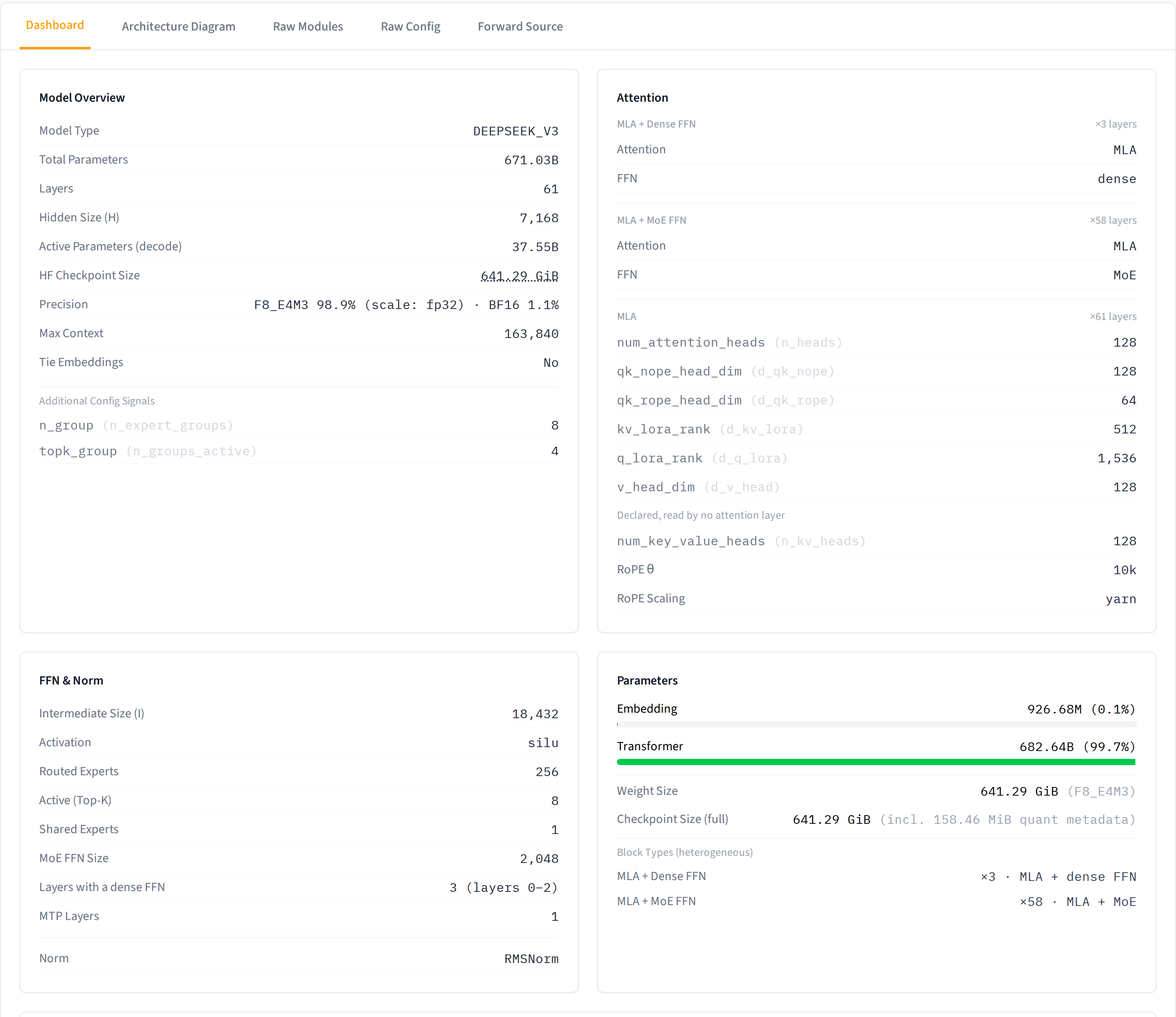
Overview panel. One screen gives the model's summary: type, layer count, hidden size, total parameters and active parameters at decode, checkpoint size and precision mix, max context. Attention is grouped by layer type with its key dimensions listed (MLA's kv_lora_rank, qk_rope_head_dim...), each dimension annotated with its symbol name in the spec. FFN and MoE show expert count, active experts, and which layers are dense. It also shows how parameters split between embedding and the trunk, and compares weight size against the checkpoint's actual bytes, which is exactly the reconciliation result from section 2.5.

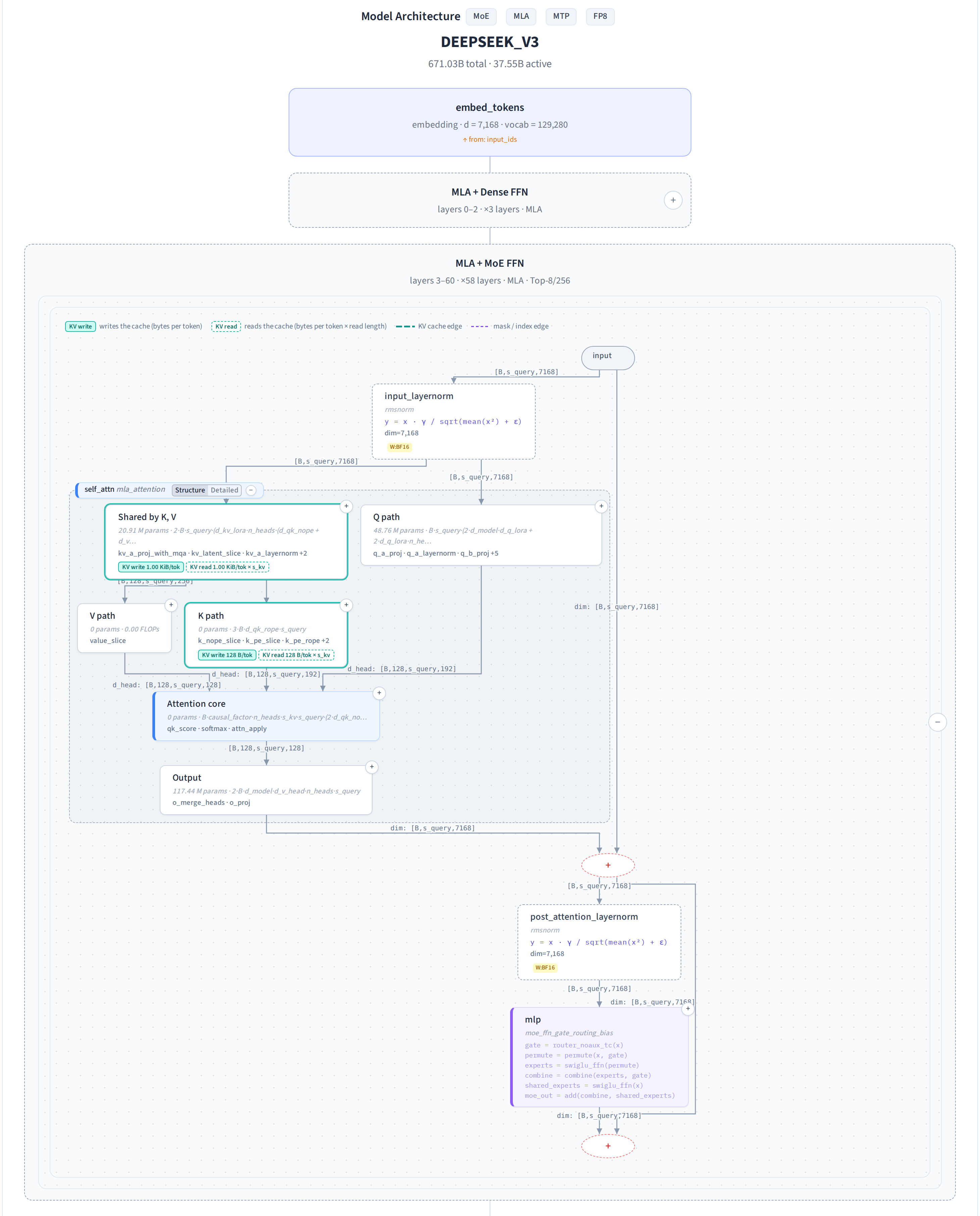
Model architecture graph. The spec is expanded into a computation graph you can open layer by layer. First you see an overview of embedding, the various blocks, norm, and lm_head. Open a block and you can see how attention, norm, MoE, and residual adds connect, with each edge labeled with its tensor shape. Open the attention, and MLA's internals are split into several paths by dataflow: the compressed latent path shared by K and V, the Q path, the K path with RoPE, the V path, the attention core, and the output projection. Each piece is labeled with its parameter count and FLOPs formula, and the cache nodes also show how much KV each token writes and reads (latent is 1.08 KiB per token, rope key is 128 B). This graph isn't a static image; it's drawn from the result of the same one evaluation.

Weight and cost breakdown. Lists parameter counts per block (attention, FFN, and experts separately), active parameters, storage bytes split by dtype and quantization scale, and per-token KV cache, with a final row totaling the whole checkpoint. Click into a specific block and you can see per-op FLOPs, bytes, and arithmetic intensity, and hovering any number shows its formula: how it was computed from the model's real dimensions. Numbers and formulas come from two bindings of the same evaluation, so they always agree.

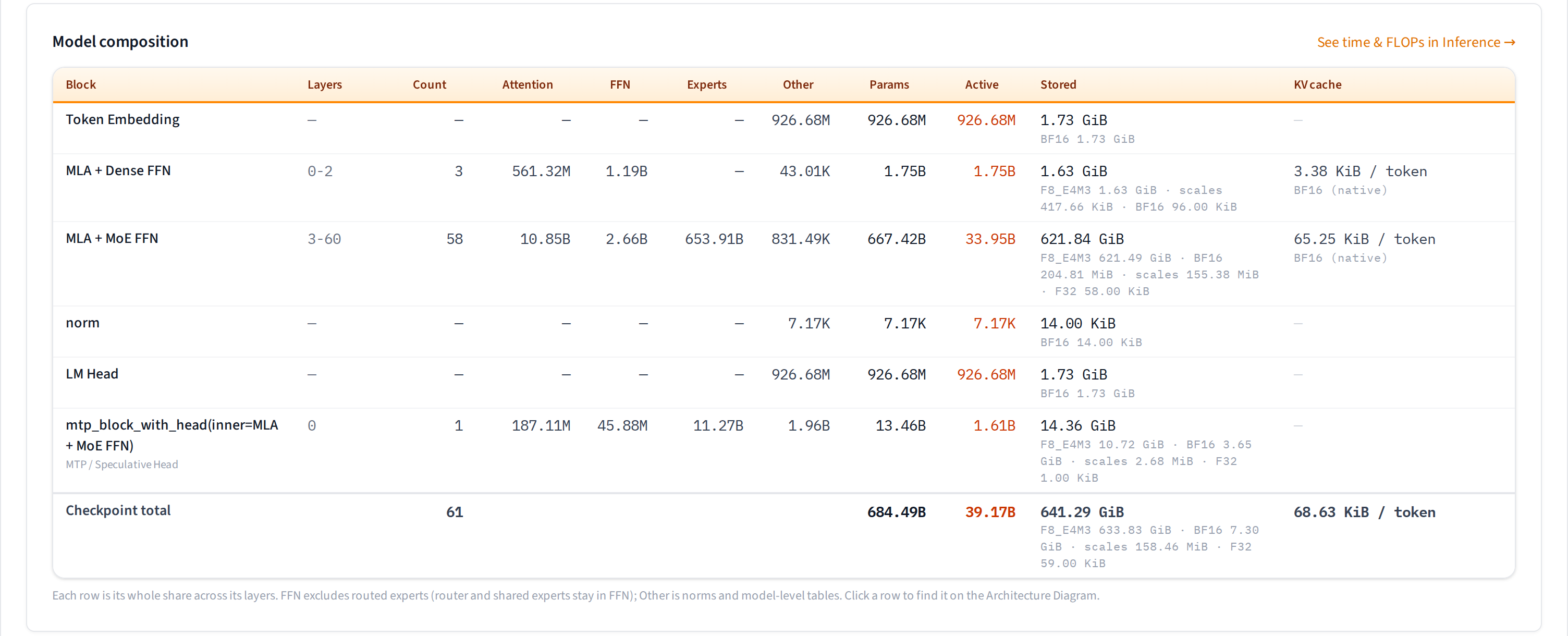
Switch to compare mode and you can put two models side by side and compare attention type, KV cache, and parameter distribution block by block. Cross-model comparison across the whole model library, and deployment cost accounting, live in the Gallery and the inference page; see Chapter 3.

---

3. Building the inference cost-accounting system

With a trustworthy spec and sympy dual-track evaluation running through all three layers, "can this model be deployed on this GPU, and how" becomes an application layer on top of the spec. No modeling code needs to change, and every number is derived from the same expression tree. The five sections below map to the five mechanism layers of this cost-estimation system: how an inference framework fuses several ops into one kernel (Fusion), how a deployment plan shards tensors across devices (parallel sharding), how to derive the shapes each device actually runs after sharding (the shape system), how SOL-based prefill/decode throughput and capacity are computed (SOL throughput prediction), and how measured data corrects the SOL upper bound into achievable throughput (driving it with a measured kernel library).

3.1 From spec to numbers: the layers of one evaluation

Before getting into the specific mechanisms, let me lay out the skeleton. A spec goes through several layers on its way to final numbers, and each layer answers only one kind of question:

Layer	What it is	What it answers
SpecIRTree	The full graph after expanding the YAML: nodes, edges, roles, cross-layer streams, layer order. The YAML is read here, exactly once	Which ops exist, and how they connect
Program	The walk schedule: which stack to walk, and whether each step is a single op or "some block × N layers". The same block template is computed once and then multiplied by the layer count	In what order to compute, and how many copies of each
Analysis	Everything you get from one walk with a deployment plan attached (parallelism, precision, batch, context): shapes, FLOPs, bytes, KV, per-GPU sharding. Numbers and formulas are two bindings of the same walk; parallel sharding is a rule propagated along the walk, not a separate graph	Every number for this run
Graph rewrite	On a copy of the Program, first insert communication according to the sharding plan, then apply fusion according to the inference framework (see 3.2, 3.3). It only changes structure and doesn't re-evaluate; the numbers still come from Analysis	Which kernels will actually run

Everything downstream (rendering, validation, capacity estimation, the Playground) reads only these layers. None of them goes back and re-parses the YAML or the raw config on its own. Each fact has exactly one origin, which is the only way numbers on different pages don't end up contradicting each other.

A small design choice inside Analysis: a set of tables, not a tree. The intuitive approach is to hang an object off every node and stuff twenty or thirty fields into it. Analysis does the reverse: it splits facts into tables by kind, each keyed by node id. One table for shapes, one for FLOPs, one for weight storage, one for quant formats, and one for "instance count", which records how many copies of this node exist in the whole model. A block template is computed once but repeats 61 times in the model; an expert is described once but there are 256 of them, with 8 active per token. FLOPs and bytes in the tables are per-copy quantities; multiply by the instance count to get whole-model totals. So asking "how many parameters does attention take in total" becomes joining the parameter table, the instance-count table, and the role table on node id, then grouping and summing, like querying a database.

The tables hold only what has to be decided on the spot during the walk: shapes and sharding state (these have to be passed down along the graph), FLOPs and cache declarations (these need to know which dims the current template is bound to), and quant formats and measured timings (these are aligned in from outside, per node). Anything that can be computed from these tables (memory-traffic bytes, KV footprint, capacity, reconciliation against the checkpoint) is never stored a second time; it's computed when needed. The KV footprint, for example, is just the cache node's shape × bytes per element × instance count, and can be computed from the tables at any time.

The reason I insist on not storing them: if a quantity can be computed from shapes and is also stored separately, nothing guarantees the two stay consistent. One day someone changes the shape derivation and forgets the stored copy, and the two quietly diverge without any error. If everything is computed from shapes, there's only one origin; wire one edge wrong and every derived number moves together. That's exactly what the claim in 3.5 that "graph errors can be detected" relies on. The full argument is in docs/evaluation_model.md.

3.2 Fusion

A spec describes the computation graph in the mathematical sense, but real inference frameworks fuse a chain of ops into one kernel: the three separate Q, K, V projections in the spec may be a single fused matmul in vLLM. HuggingArch models "how the framework fuses" explicitly as a table: each fusion rule describes an op topology that can be merged, and each framework (vLLM / sglang, per version) declares which rules it actually enables. These rules were compiled one by one from the vLLM and sglang source code.

Fusion has two subtleties:

• It comes after communication. A fused kernel has no cost formula of its own; its FLOPs and memory traffic are simply the sum of the ops it absorbs. And communication itself can get fused in too, e.g. an all-reduce and the RMSNorm right after it combined into one kernel. So communication has to be inserted per the sharding plan first, and fusion happens after that.
• It depends on conditions, not just topology. Even when the ops are wired the right way, the framework doesn't necessarily fuse them. For example, for Qwen3-MoE attention sglang can combine QK-norm and RoPE into one kernel, but only when head_dim is 64, 128, or 256, RoPE covers the entire head, activations are BF16, it runs on CUDA (and the corresponding launch flag is on). Otherwise it's still several separate kernels. These conditions are written next to the fusion rule, and matching checks them against the actual dims, precision, and GPU of this evaluation. Likewise, prefill and decode may walk different subgraphs to begin with (e.g. MLA switches to the absorbed variant in decode), so each phase is fused separately.

Fusion only changes the graph's structure; the numbers still come from the same evaluation. In the UI, the Inspector draws the pre-fusion graph, the inference page's computation graph draws the post-fusion graph, and expanding a fused node shows which ops it absorbed; the Fusion page lists which rules a given model hits on a given framework and version. That way the spec doesn't stop at a "theoretical op graph" but also lines up with "how this framework, at this version, will actually run it".

3.3 Parallel sharding: sharding is state propagated along the graph, and communication is derived

Putting a model on multiple GPUs means a combinatorial explosion of ways to shard it: attention split 8 ways by head, MoE experts spread over 32 GPUs, another layer of CP for long context, and PP between layers. Hand-writing "where to shard, where to communicate" for every model and every combination would never end, and there'd be no way to guarantee it's right. The most naive "total ÷ number of GPUs" is even worse: it can't tell you which tensors share a communication group, nor which edges need communication inserted.

HuggingArch borrows the idea from PyTorch DTensor (and its origin, GSPMD, Xu et al. 2021): sharding is a state of a tensor, and like shape, it propagates down the graph. On each parallel dimension, every tensor is in one of three states:

• Sharded: each GPU holds only one slice;
• Replicated: each GPU holds a full copy;
• Partial: the shape is complete, but the values on each GPU are only a partial sum; you have to add them up to get the true value.

Partial is the key to the whole design: it has exactly the same shape as a complete tensor, so you'll never spot it by looking at shapes alone. Only by propagating state all the way down do you know that what the downstream op receives still "owes a sum".

Let's walk through one layer of TP attention:

q_proj      weight split by head (column-split)   → output: Sharded by head
attention   each GPU computes only its own heads  → output: Sharded by head
o_proj      weight split by head (row-split)      → output: Partial (one partial sum per GPU)
+ residual  residual add needs the full value     → states don't match → all-reduce inserted automatically

Nobody ever wrote "o_proj is followed by an all-reduce" in the spec. The spec only writes dims (o_proj's input is n_heads * d_head), and the dimension table says the head axis is sharded by TP; the row-split produces Partial, the downstream wants Replicated, and the difference between the two is one all-reduce. Communication isn't written down; it's derived from the state difference. The same rule applies elsewhere: Sharded meeting a reader that needs the full value derives an all-gather; tokens that need to reach experts on other GPUs derive an all-to-all; under CP, each GPU computes attention over its own segment of KV, and merging them derives a log-sum-exp reduction. TP, EP, and CP aren't three mechanisms; they're the same state algebra applied to different edges.

There's a question hidden in that walkthrough: q_proj's output is one flat n_heads × d_head feature axis. After it's split by head, it goes through several reshapes (splitting heads, transposing, scoring, merging heads). Why should the sharding state still "keep up"? The answer is each op's DimMap, the same per-axis correspondence table that shape inference uses in 2.4. It says where each output axis comes from in the input: carried over as-is, split out of one axis, merged from several axes, or newly created. Sharding follows that table:

q_proj output  [B, s, n_heads·d_head]      sharded on the last axis (by head)
split heads    [B, s, n_heads, d_head]     this axis splits in two; sharding lands on the "head count" part, d_head stays whole
transpose/score [B, n_heads, s, s]         head axis carried over as-is, sharding follows; d_head is contracted away, irrelevant to sharding
merge heads    [B, s, n_heads·d_head]      axes merge; sharding returns to the merged axis

There are only a few rules: when an axis is carried over as-is, sharding follows it; when one axis splits into several, sharding lands on the outermost part (whole heads are distributed); when several axes merge, sharding follows to the merged axis; when an axis is contracted away, its sharding goes with it. Shape inference and sharding propagation read the same table, so as long as an op's shape is right, its sharding is right too; there's no need to write a second set of sharding rules per op. The table works by axis position, not axis name, so a head axis hard-coded as 64 and a head axis named n_heads are handled exactly the same way.

This approach also derives some "counterintuitive" conclusions on its own. MLA caches a compressed latent, which has no head axis at all, so TP can't shard it: every GPU has to store a full copy, and raising TP does nothing for MLA's KV footprint. To spread it out you need attention data parallelism, with different GPUs handling different requests. That's not a special case for MLA; it's read straight off the dimension table. EP falls out just as naturally: it doesn't shard an expert's shape, it only reduces the number of experts on each GPU (the instance count), with each expert staying whole. Sharding inside an expert is TP's job; the two multiply, and "EP + TP" needs no special logic.

Derived communication is a real node on the graph: it appears in the per-op cost table with its own communication bytes, is priced on intra-node high-speed links or the inter-node network according to the topology of its communication group, and can take part in the fusion from 3.2 (all-reduce combined with the following RMSNorm into one kernel). PP is the same: the repeated layers are cut into a few contiguous segments, and any edge crossing a segment boundary becomes a point-to-point send. Not just the main hidden state, either: cross-layer streams (like the top-k selection DSA shares) are automatically counted when they cross segments.

Finally, per-GPU shapes, FLOPs, and memory are all "read" from the same evaluation according to sharding state, not re-evaluated for each sharding scheme; dim lengths always stay global. This gives a property you can write as a test: the two CP schemes (Ulysses and pcp) communicate differently, but each GPU holds the same data, so per-GPU memory-traffic bytes must be equal. That's exactly what the test asserts. The full rules are in docs/parallelism.md.

3.4 SOL-based prefill / decode throughput prediction

The Intro gave the SOL time of a single op, $T_{\mathrm{SOL}}=max(\text{FLOPs}/\text{peak compute},\text{bytes}/\text{bandwidth})$. The inference page extends it to a whole deployment and answers three questions: does it fit on each GPU, how long does one step take, and how big a batch can it run. The inputs are the parallel plan from 3.3 and a GPU spec table (memory, bandwidth, peak compute; adding a GPU is adding one row).

This layer doesn't depend on any kernel measurements. What it gives is the lower-bound time set by the hardware roofline, which no implementation can beat. Under the same yardstick, different parallel plans, different GPUs, and different models can be compared directly, without interference from how good or bad a kernel implementation happens to be. That's exactly the core need behind the "cost accounting" in the Intro.

Below, using DeepSeek-V3 on 8 B200s (attention data parallelism + expert parallelism, 1024 input and 1024 output tokens) as the example:

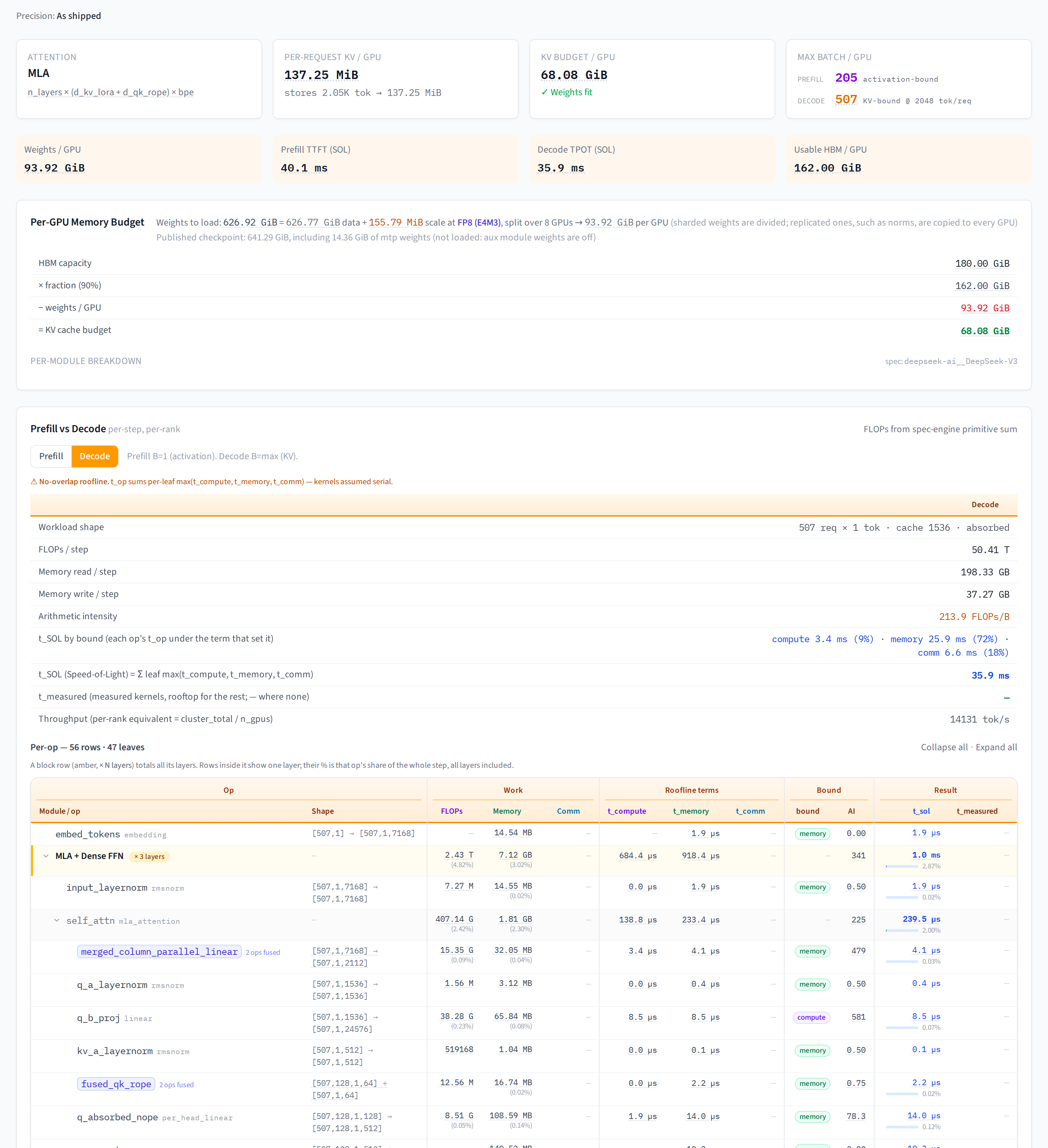
Memory: weights first, the rest goes to KV. Each B200 has 180 GiB; at 90% usable that's 162 GiB. Weights spread across GPUs per the sharding plan come to 93.92 GiB per GPU. The byte counts come from the storage table in 2.5 that was reconciled against the checkpoint, with FP8 weights, the small amount of BF16, and quant scales each counted on their own. The remaining 68 GiB is the KV cache budget. KV is accounted according to each cache tensor's own growth law: GQA's K and V grow per token, MLA stores only the compressed latent plus one shared rope key, sliding windows cap at the window length, and the recurrent state of linear attention and SSMs doesn't grow with context. A single layer can also carry several caches with different laws at once (one DeepSeek-V4 layer has sliding-window KV, compressed KV, and indexer keys, each counted separately; the full model is in docs/kv_cache_storage.md). In this example, KV per request is 137 MiB, decode fits at most 507 requests, and the bottleneck is KV; prefill's batch is capped first by activations, at only 205.

Time: take each op's bottleneck, then sum. For each op, three terms are computed (compute time, memory time, communication time), and the largest becomes its SOL; one step's time is the sum over all ops, with no assumption that kernels overlap. That's where the per-op table in the lower half of the figure comes from: each row marks whether the op is compute-bound or memory-bound and its arithmetic intensity, and fused kernels (3.2) and inserted communication (3.3) each get a row too. Summed up, in this configuration one decode step takes 35.9 ms: 72% of the time goes to memory access, 18% to communication, and only 9% to compute, a textbook bandwidth-bound case. TTFT is 40.1 ms, which works out to about 14,000 tokens/s per GPU.

Sweeps: one point isn't enough, you need curves. The Scaling panel at the top of the inference page sweeps the same estimate along several axes: fix 4K context and sweep expert parallelism from 4 GPUs to 256, comparing per-GPU throughput across GPUs; fix 8 B200s and sweep batch × context length to see how prefill and decode throughput change; and separately look at how per-request KV grows with context and how many requests fit on one GPU. Points beyond the model's published context limit (163,840 for V3) are clearly marked: they're extrapolations, not a range the model can actually serve.

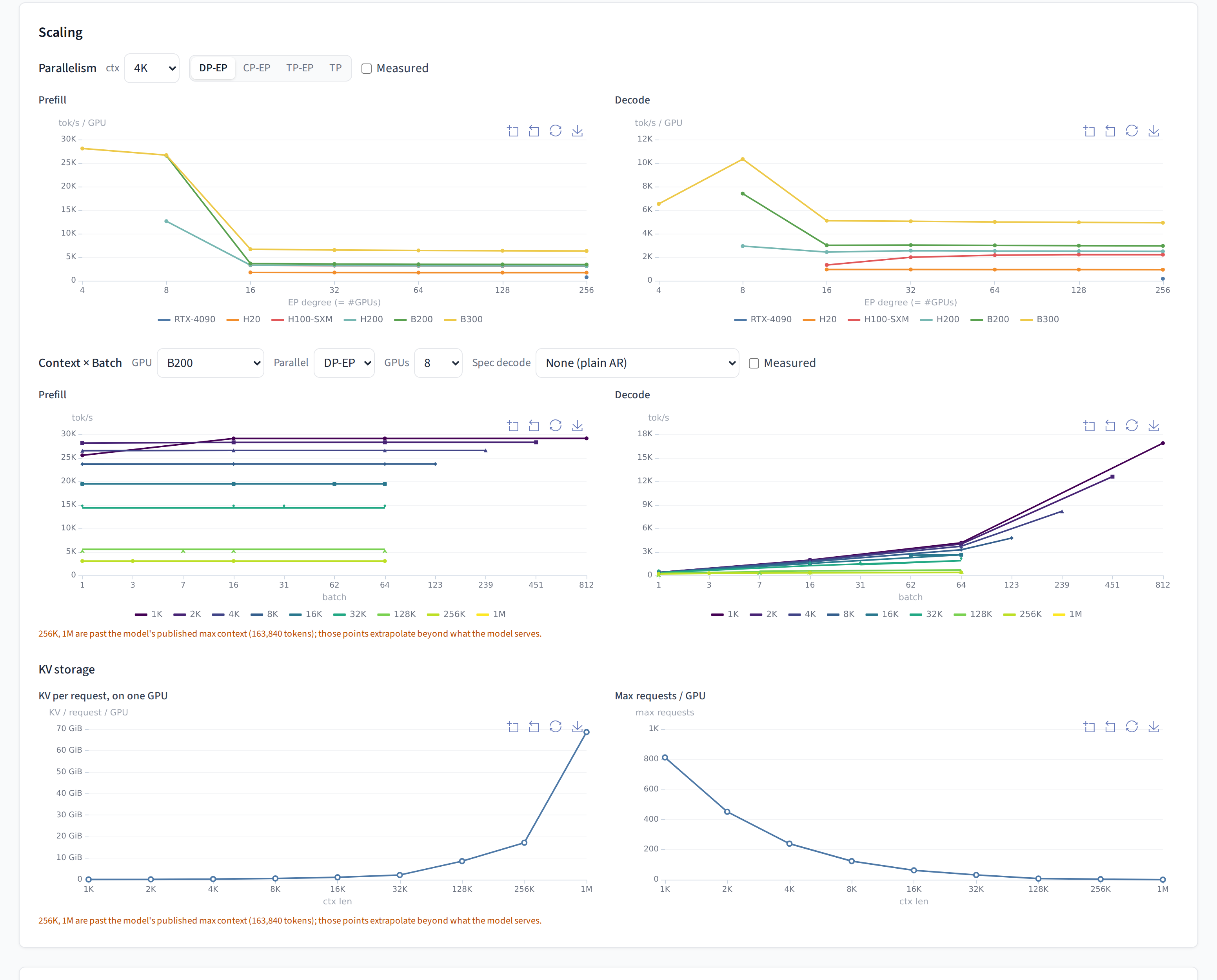
All of the above is pure SOL, without a single kernel measurement. Real kernels only reach part of the upper bound; the next two sections cover how measured data corrects it to achievable throughput. But that doesn't change SOL's role as the baseline for comparing across models and plans.

3.5 The shape system: every derived quantity shares one shape derivation

Looking back, the entire cost-accounting system rests on just two basic facts: parameter counts follow the actual shapes of tensors in the checkpoint, and every other derived quantity comes from the result of one shape propagation. FLOPs take their dims from the actual axis lengths propagated to that node; HBM read/write bytes are computed from tensor shapes on each edge (the intermediates saved by fusion are also read directly from the shapes at the fusion boundary); KV cache expands with shape according to each cache tensor's own storage law; per-GPU geometry is derived from the layout carried along this walk, with dim lengths kept global, instead of dividing the parallel degree into the binding and re-running a graph. We deliberately don't maintain a second, independent computation path for any derived quantity. Early versions did have them (a per-module-category lookup table of sharding factors, a side path that counted FLOPs from environment dims), and in practice they all gradually drifted from the shape derivation as the code evolved, and that drift never triggered any error.

After converging FLOPs onto shape derivation as well, an unexpected benefit appeared: many spec graph errors show up as detectable numeric or geometric discrepancies. For example, mistakenly building a grouped einsum as a dense fully-connected layer, wiring the axis order of a 4D tensor backwards, or connecting lm_head's input edge to a scalar gate can make FLOPs, byte counts, or shape diagnostics deviate. We found and fixed errors like these in the DeepSeek-V4-Pro and Kimi-K3 specs, in each case judged against the actual shapes of the corresponding tensors in the checkpoint. But this isn't a completeness guarantee: shape checks only prove that the tensors fit together, and the repo has no checker covering all equivalent topologies.

From deployment plan to the real per-GPU shapes

To correct the SOL upper bound toward a real implementation, the first step is knowing the shape each op actually runs at on each GPU, which needs a reliable shape system. It reuses the same mechanism as the shape inference in Chapter 2: the walk still computes shapes at global lengths, the layout records on each edge which block each GPU gets, and local shapes are derived at read time, not by binding a second set of divided dims and evaluating again.

Concretely, a valid deployment plan (ParallelConfig) decides which axes are split by which process groups: attention's n_heads belongs to TP, as do the dense / expert intermediate dims, and EP splits the number of expert copies n_expert_copies without touching the routing denominator n_experts. Dim lengths stay global; how much each GPU gets is a cell the layout hands out at read time, not something divided into the binding before evaluating again. LayoutPropagation records each edge's layout along the walk, and local shapes, FLOPs, and memory traffic are derived from the same Analysis. This is the core of "one walk, with layout handling per-GPU": no separate derivation logic has to be written for arbitrary TP / EP / CP combinations.

The shapes obtained this way are the real sizes executed on each device. For example, for DeepSeek-V2-Lite under tp_ep8, grouped_gemm's K is 1408, which can be fed directly into the measurements in the next section. Its use complements the shape inference of Chapter 2: Chapter 2 uses it as a geometric consistency check while building the spec, while here it's used to derive forward from a deployment plan to the real kernel shapes on each device. Details of the placement algebra are in docs/parallelism.md.

A reliable shape system brings one more key benefit: since it can derive the real per-GPU kernel shapes under a distributed deployment forward from the deployment plan, you only need to profile an op at that shape on one GPU to get kernel performance that would normally require actually standing up a large distributed cluster to measure. In other words, the lightest-weight single-GPU measurement covers the op costs of a distributed deployment. That's also the premise for the measurements in the next section.

3.6 Driven by a measured kernel library: correcting the upper bound to what's achievable

SOL is an upper bound. Real kernels only reach part of peak, and which kernel is fastest depends on shape, dtype, and the library used. 3.4 answers "how fast could it be at best"; this section answers "how fast is it actually today".

The reference isn't any one framework, but the fastest correct kernel in the whole ecosystem. For the same op, FlashAttention 2/3, FlashInfer, FlashMLA, DeepGEMM, FLA, Mamba-SSM, vLLM, and sglang often each have their own implementation. HuggingArch doesn't favor any of them: each op category defines a mathematical contract specifying what it has to compute; each library's kernel registers under that contract as an adapter, declaring which shapes it supports and how to convert the standard inputs into its own layout. At measurement time, every applicable kernel runs on the same shape. A new kernel coming out is just one more row of data.

Correct first, then fast. Every contract comes with a reference implementation written in PyTorch eager. After a kernel's output is converted back to the standard layout, it's compared to the reference with a dtype-dependent tolerance (loose for FP8, medium for BF16, strict for FP32), and if it doesn't match it isn't recorded. "Fastest" can't be won by a kernel that computes the wrong answer. Numbers that survive also go through a physics check: the compute utilization (MFU) and bandwidth utilization (MBU) derived from them can't exceed SOL; if they do, it can only mean the measurement itself went wrong.

What's measured is the shape that actually runs on each GPU. 3.5 derived the real shape of every op on every GPU forward from the deployment plan, and the measurement plan is generated directly from there: given a model and a set of batch / context values, list all the kernel shapes one real inference would hit, deduplicate, and measure them one by one on a single GPU. So kernel costs under a distributed deployment don't require actually building a cluster to measure. (Collectives are the exception: they inherently need multiple GPUs and aren't in this single-GPU pipeline yet.)

Measured and SOL side by side, neither overwriting the other. Measured time sits next to SOL in the per-op table from 3.4: readers see the upper bound and also how far today's implementation is from it. By default it takes the measured value of the selected inference framework's own kernel at the newest version in the corpus, noting which version; you can also switch to "envelope" mode, which takes the fastest kernel from any library. Ops without measured data keep using SOL.

The list of supported libraries and kernels is in docs/measured_calibration.md.

3.7 Kernel Bench: turning kernel benchmarking into a database

I think a database-centered Kernel Bench is meaningful in its own right. In practice you're constantly benchmarking kernels, but the results tend to lie scattered across docs, spreadsheets, and chat logs: what shape was measured, what dtype, which library version, on which GPU. It's hard to say after the fact, let alone put side by side with someone else's results.

HuggingArch gives every test a complete workload signature: op type, the shape this op cares about, dtype, GPU, prefill or decode, parallelism, plus library name, version, and kernel name. With that signature, all test data can be stored, queried, and compared systematically, like rows in a database. The whole flow goes like this:

1. Generate test targets. Export a test plan from a model and a set of batch / context values, i.e. all the kernel shapes one real inference would hit (see 3.6).
2. Benchmark locally. The hbench CLI prepares an isolated environment for each kernel library on your own machine (different libraries' dependencies often conflict), and calls the corresponding provider to benchmark each one; every result row is stamped with the library version actually installed. The version is part of the data, and results are append-only, never overwritten.
3. Validate. Each result is first compared numerically against the reference implementation, then checked for MFU / MBU exceeding the hardware limit; results that fail never leave your machine. After upload, the cloud computes it again and flags anomalous rows.
4. Upload and manage. Uploaded data is private by default and only calibrates your own estimates; if you want to contribute it to everyone, submit it for review, and once an admin approves it gets merged into the shared corpus. The web UI lets you browse, filter, and visualize all historical data.

This way, all implementations of the same op can be compared side by side, and so can the same kernel across different framework versions. Kernel benchmarking no longer needs someone running and recording it by hand over and over: kernel developers can focus on optimizing the kernels themselves, and inference engine developers can find the current best implementation right here. Full CLI usage is in kernel_bench/README.md.

---

4. Model Arch Design: designing models on top of the spec

The spec breaks a model into reusable components, so HuggingArch can do more than analyze existing models: it can also answer "what if I swapped out this module?" The Playground offers two ways to play with that. You can line up several modules that fill the same position and compare them side by side, or you can start from an existing model, replace some of its modules, and watch how the whole model's numbers change. In both cases the numbers come from the same evaluation as the Inspector and the inference pages, not from a separately written estimate.

4.1 Module comparison: one position, five attentions

Attention is where most of the creativity has gone in the last couple of years. Take DeepSeek-V3's MLA, DeepSeek-V3.2's DSA, DeepSeek-V4-Pro's CSA and HCA, and Kimi-K3's KDA, and put them in one comparison table. Each module binds its internal dimensions (head count, latent width, window, compression ratio, ...) the way they are in the original model, and then all of them are compared under the same fixed contract: the same hidden size (7168), batch, sequence length and GPU. So what's being compared is "the cost of dropping it as-is into the same position," not a ranking of architectures.

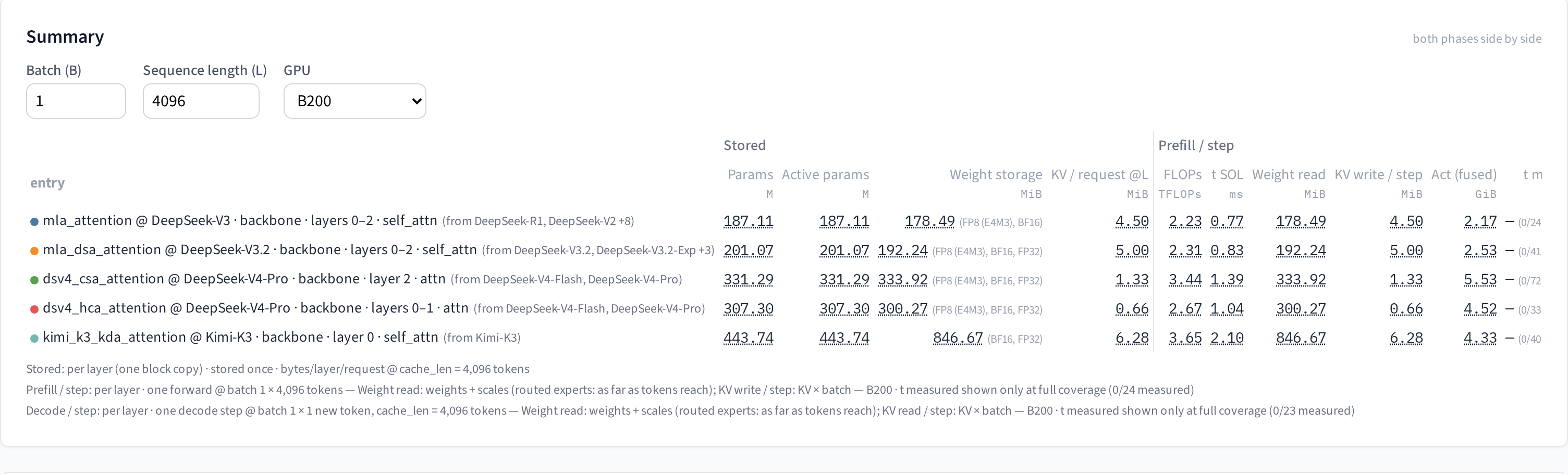
Looking only at per-layer parameters and prefill time at 4K context, MLA is the cheapest (187M parameters per layer, 0.77 ms) and KDA is the heaviest (440M, 2.1 ms). What really separates them is how the KV cache grows with context:

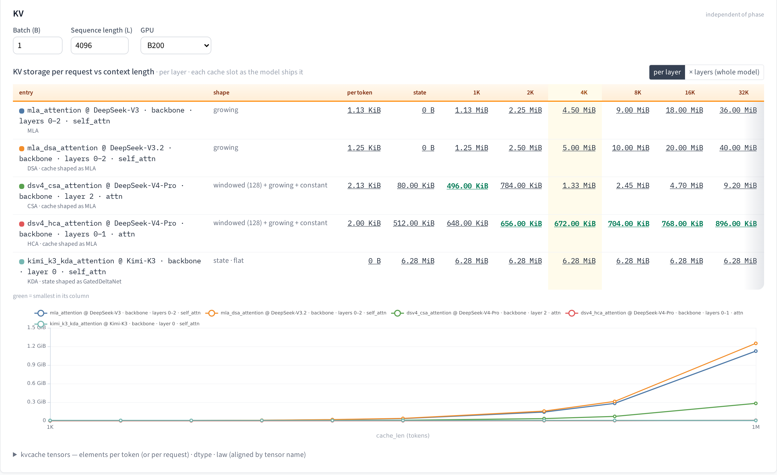
At 32K context, the KV per layer per request is: MLA 36 MiB, DSA 40 MiB, CSA 9.2 MiB, HCA 0.9 MiB, and KDA a constant 6.28 MiB. The table lays out the trade-offs of these designs very clearly:

• DSA does not save KV. On top of MLA's latent, it stores an extra set of index keys. What it saves is compute: a very light indexer first scores every token, and the main attention only looks at the top-k of them, so at long context the bulk of attention cost no longer grows quadratically with context.
• CSA and HCA save the KV itself. Both keep a 128-token sliding window and store earlier tokens compressed along the time axis. HCA compresses harder; at 32K it's still under 1 MiB.
• KDA is linear attention. It stores a fixed-size recurrent state that doesn't grow with context. So at short context it's actually the most "expensive" (6.28 MiB at 1K, where MLA is only 1.13 MiB), but past a few thousand tokens it pulls ahead and stays there.

You can also compare where two modules differ structurally. Below is the compute-graph diff of MLA and DSA. Nodes in the two graphs are paired by declaration, not by name; nodes present on both sides but with different attributes are outlined in orange, and paths that exist on only one side are marked separately:

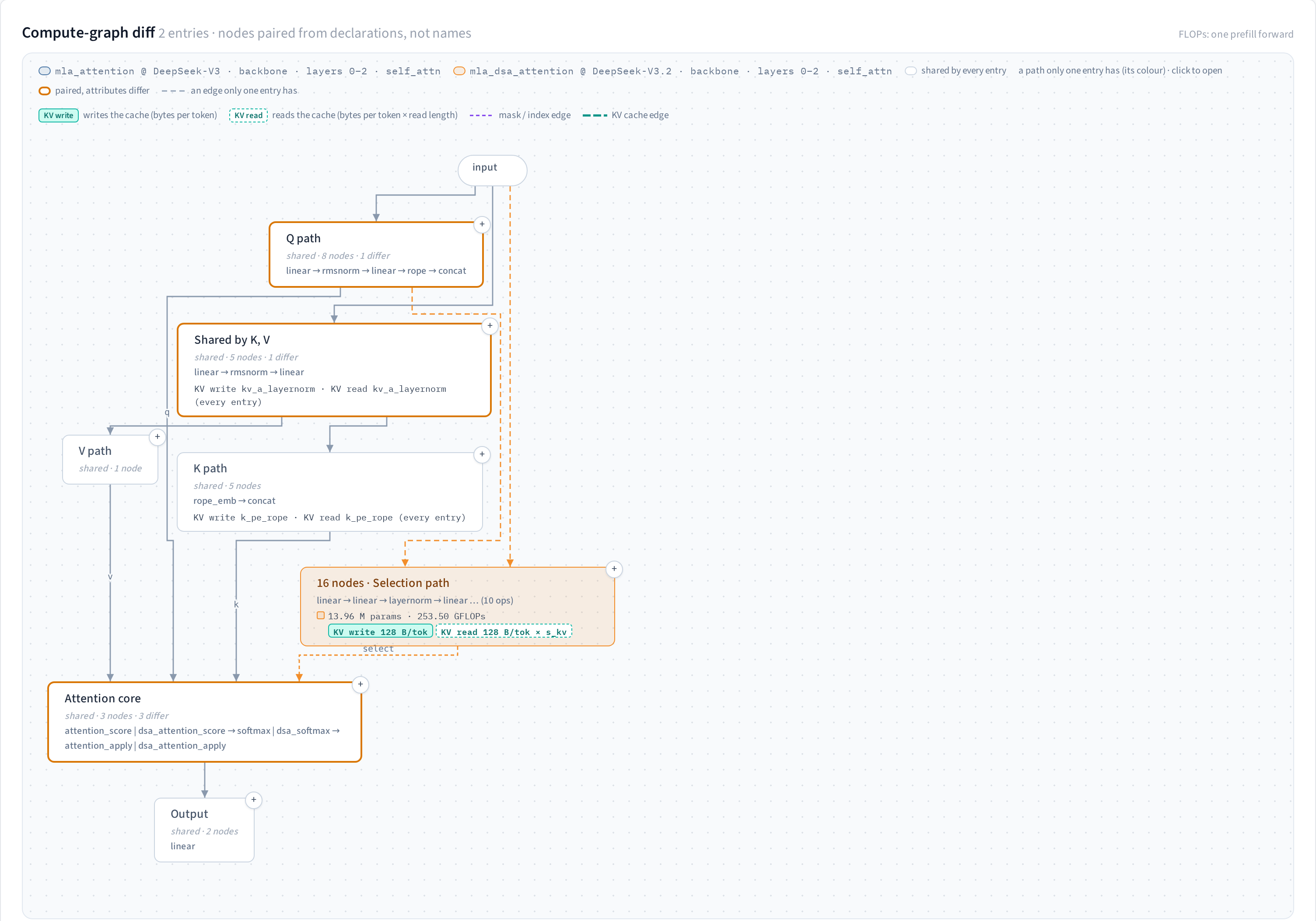
You can see everything DSA adds at a glance: a 16-node selection path (that's the lightning indexer), which writes its own index cache at 128 bytes per token and then tells the attention core which tokens to look at through a select edge.

4.2 Starting from an existing model: swapping V3's MLA for DSA

Module comparison answers the per-layer cost. If you want to know what the whole model looks like after the swap, use the Model Editor. Load DeepSeek-V3, and it splits into layer groups: the first 3 layers with dense FFN, the next 58 with MoE, plus an MTP head. Swap the attention of the first two groups from mla_attention to mla_dsa_attention, and that's essentially the DeepSeek-V3.2 structure.

After the swap, the editor doesn't quietly fill in defaults. It tells you outright: DSA needs three dimensions MLA doesn't have (index head dim, number of index heads, top-k), please bind them. Fill in V3.2's values (128, 64, 2048) and the whole model gets recomputed, with each group's parameters, FLOPs and weight bytes shown as "old → new":

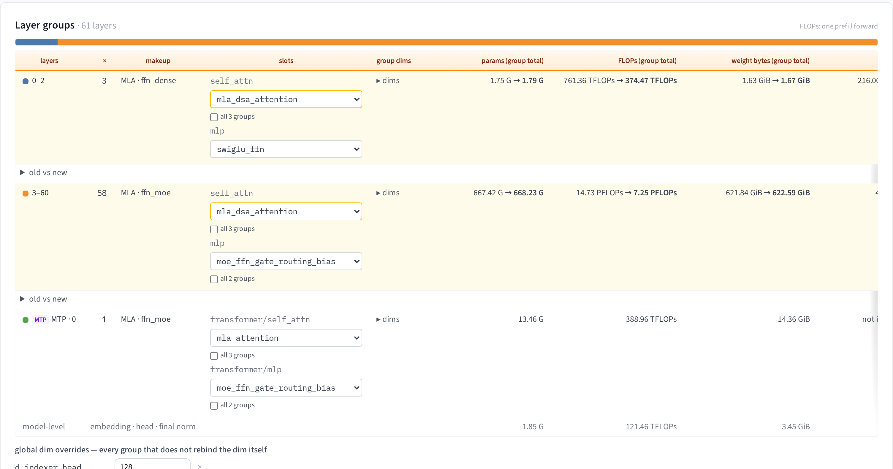
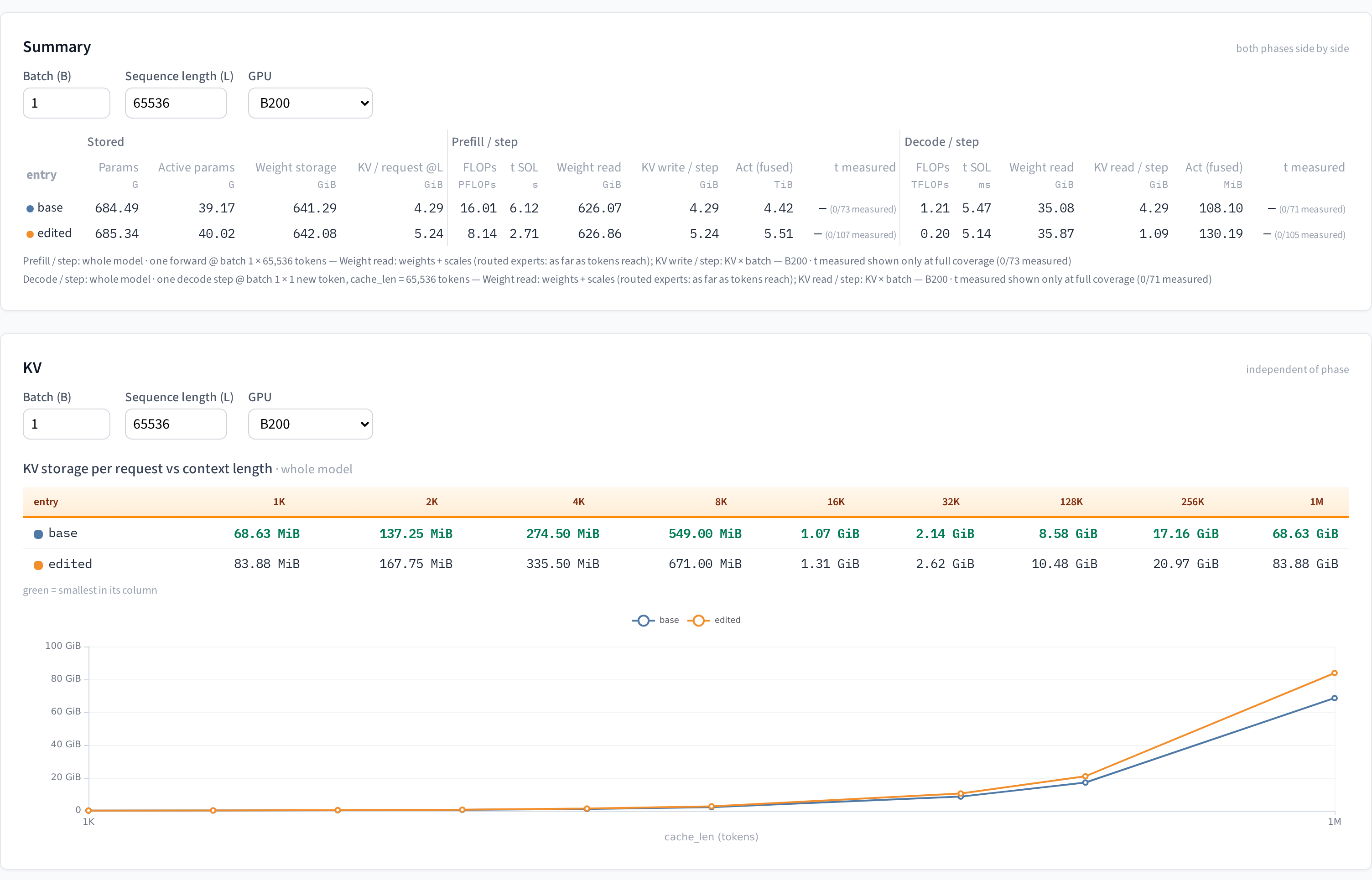
At 64K context, single request, on B200: prefill FLOPs drop from 16.0 PFLOPs to 8.1, and SOL time drops from 6.1 s to 2.7 s; the KV read per decode step drops from 4.29 GiB to 1.09 GiB. The price is about 850M extra parameters (the indexer's weights) and about 22% more KV per request (the index keys). That is exactly the trade-off DeepSeek made going from V3 to V3.2. And here, without writing a line of code or training a model, you can do the math in a few minutes.

---

5. Some lessons from vibe-coding a large project

The first POC of HuggingArch came together fast. But it took patching and mending all the way up to the National Day holiday to drag it into presentable shape, and nearly three months of that went into refactoring. Here are a few lessons from writing a large project with agents.

Get the architecture layering clean first

If you want a framework you can actually maintain, the first thing you need is clean layering. HuggingArch is a project about "computing numbers," and the easiest mistake for an agent to make is to patch things in place: some page's numbers don't match, so it recomputes them inside the page; some model has a problem, so it adds an if model_id == .... Each patch looks reasonable on its own, but once they pile up, different pages give different answers about the same thing. That's the most common bug in this project: not wrong logic, but two places each doing their own math.

So the first rule of the repo is: every number comes from a single source in the backend. The spec is expanded once and evaluated once, and rendering, validation, capacity estimation and the Playground all read only that one result. If a fact is missing, you first compute it in the evaluation and store it as a field, then read it; downstream code is not allowed to derive it on its own. The second rule is no ad hoc fixes: when you see a bug, first ask what class it belongs to and whether it shows up elsewhere too, and fix the abstraction, not the one case that triggered it. Writing this in a doc isn't enough; the key rules all need tests guarding them. The dependency direction between modules is hard-checked by a test that scans imports, and crossing the line turns it red. Every place where "downstream derives facts on its own" has been counted one by one into a scoreboard that is only allowed to go down, never up.

CLAUDE.md: the repo rules every agent shares

CLAUDE.md matters a lot. Every new session, whether it's Claude, Codex or Kimi, starts out knowing nothing about this repo, and CLAUDE.md is their common entry point: how the project is layered, which invariants must not break, what to change when adding an op / quant scheme / GPU model, how to run the tests. Give CLAUDE.md enough information, architectural principles and coding conventions, and every time a session restarts the model can catch up quickly instead of making inefficient back-and-forth changes.

Two-reviewer review: one writes, two review

No matter how good the model is, it will make mistakes when designing a complex feature, and it's hard for it to catch its own. My approach is "three-party review": cut the change into small steps that can each be reviewed on their own. Each step is implemented by one agent, and then two different agents review it in parallel. One reviews the implementation: it compares old behavior branch by branch and runs its own measurements instead of trusting only the tests the implementer ran. The other reviews the design: does the implementation match the plan that was signed off beforehand, and how should any new trade-offs that came up during implementation be settled? Only when all three sign does it merge into main; if one doesn't, the implementer fixes it and only that party re-reviews. Roles aren't tied to specific models. Claude, Codex, Kimi, Grok can each take any role. Different models have different blind spots, so cross-review complements them nicely.

Once this process is running smoothly, you can let it push forward batch after batch unattended: if both sides sign, it merges automatically, and only uncertain things, like changes to golden data or calls that need product judgment, are left for a human to decide.

This Ralph-loop idea of having the models spar with each other turned out to be really useful. Early in the refactor, Opus would often introduce new hacks while refactoring away old ones, and weeks of old-school manual vibe-wrestling with the model got me nowhere. Once I had the strong model design and write, and a runner-up (Chinese) model review, the project moved forward steadily and in order, which largely solved the hard problems I hit during the refactor.

So as a coder in 2026, you need both SOTA tokens and cheap tokens!

Roadmap

HuggingArch is still an evolving scaffold. A few directions for what's next:

• Correctness checks and fixes for existing models: there are a lot of models, and it'll take time to analyze them more carefully and verify the results. The numbers for some common models have been checked through observation and manual review and look solid, but one pair of eyes can't cover everything, and new models keep coming in, so over the coming months I'll probably verify correctness along the way through manual analysis.
• More precise inference modeling: building on the existing speculative-token and ep_load_factor parameters, add more scheduling detail, and calibrate theoretical comm time against more measured communication numbers, so the estimates get closer to real deployments.
• A thicker measured corpus: expand the GPU models, op libraries and models covered by the measured corpus. Every additional measurement narrows the SOL upper bound a bit more toward achievable throughput.
• A more complete model design workflow: the repo already supports importing custom models; the next step is to make editing, comparison and feedback during architecture design into a more complete interactive loop.
• Training cost modeling: extend cost modeling from inference to training. Is this even possible? (PP bubbles maybe not, but memory planning should be pretty easy.) Happy to discuss, come find me.

How to contribute

This is an open, side-project-style project. Stars are welcome, and so are developers who want to build it together. Ways to get involved:

• Contribute model specs: run the agentic generation pipeline for a model that isn't supported yet. Publishing to the cache re-requires validate() to return valid: true, which includes model_storage_bytes.diff == 0. You then run Review on your account page, and after it PASSes you Open PR yourself; the service creates the spec bundle PR through a GitHub App. Fill in your GitHub handle in your profile and the PR commit will carry a Co-authored-by trailer. Promoting a new draft component is a separate maintainer process.
• Contribute measured corpus data: run kernel_bench on your own GPUs and upload the measured CSV. This data immediately calibrates your own estimates (no need to make it public), and you can also nominate it into the shared corpus, where after review it becomes a public baseline visible to everyone.
• Contribute components and fusion bindings: a new topology component goes through components/drafts/ → review → backend.arch.promote; fusion plans / framework bindings are submitted through the normal code review process for their registry.
• Report problems, join the discussion: if any number doesn't add up, or some new architecture isn't supported yet, issues / PRs are very welcome. [Crowdsourcing bug fixes beats fixing bugs alone!]

For getting started and the code structure, see the repo's docs/ (README.md is the map of the layers); for mechanism details, see the individual deep-dives.

Citation

If this project or post helps your work, you can cite it as:

@misc{shen2026huggingarch,
  author       = {Shen, Han},
  title        = {HuggingArch: Automating Model Architecture Analysis},
  year         = {2026},
  howpublished = {\url{https://shenhan.cc/blog/huggingarch}},
  note         = {Code: \url{https://github.com/shenh10/HuggingArch}}
}

Acknowledgments

I thank my advisor, Prof. Wei Xu, for providing the H100 and RTX 4090 GPUs this work ran on, and for his hands-on support in keeping those machines running. This project would not have reached its current form without him.